XGBoost Introduction

This article will deal with one of the implementations of Gradient Boosting Algorithms- XGBoost Algorithm. Since its inception in 2014, XGBoost has always been a lauded algorithm for implementing Machine Learning models. The algorithm has a wide range of applications ranging from predicting ad click-through rates to the classification of high energy physics events. Known for its speed and accuracy, XGBoost is an implementation of gradient boosted decision trees.

In this PythonGeeks article, we will guide you through the nitty-gritty of this algorithm. We will look at what exactly this algorithm is and why we should use ensemble algorithms to implement it. We will also look at the prerequisites for XGBoost as well as the reasons for choosing it as your first preference for any Machine Learning model. Towards the end of the article, we will go through the features of the XGBoost. So, let’s quickly get to the introduction section.

What is XGBoost?

XGBoost is an acronym for eXtreme Gradient Boosting. Developed by Tianqi Chen, it is an implementation of the gradient boosting algorithm. It is one of the most widely used tools amongst the various other tools available for the Distributed Machine Learning Community, more commonly referred to as DMLC. It is an ensemble learning method.

When asked about the difference between XGBoost and other gradient boosting algorithms, the developer Tianqi Chen gave a brief answer stating the reason that the name XGBoost actually means engineering goals to push the limits of the computational power of the resources available for boosted tree algorithms. This precisely states the reason for choosing XGBoost over any other algorithm.

Since it is a widely used algorithm, the majority of the interfaces support XGBoost for implementing Machine Learning Models. It is a typical software library that you can download and then install on your device along with any of the interfaces that we have mentioned below:

• Command Line Interface (CLI)
• Scikit models as well as Python Interface
• C++ (The actual language in which the algorithm is developed)
• Julia
• Java and JVM languages like SCALA.

History of XGBoost Algorithm

XGBoost initially started as a research project by Tianqi Chen as part of the Distributed (Deep) Machine Learning Community (DMLC) group. Initially, it began as a terminal application that could be configured using a libsvm configuration file. It became well known in the ML competition circles after its use in the winning solution of the Higgs Machine Learning Challenge. Soon after, the Python and R packages were built, and XGBoost now has package implementations for Java, Scala, Julia, Perl, and other languages.

While the XGBoost model often achieves higher accuracy than a single decision tree, it sacrifices the intrinsic interpretability of decision trees. For example, following the path that a decision tree takes to make its decision is trivial and self-explained, but following the paths of hundreds or thousands of trees is much harder.

Why prefer Ensemble Learning?

As we have seen in the introduction section, XGBoost is an ensemble learning method. In some cases, it becomes difficult for us to just go with the results of a single Machine Learning Model since the possibilities of errors are quite high. Like gradient boosting, Ensemble Learning also provides a method in which we can combine the predictive power of multiple learners giving us a solution for our problem.

This results in the development of a single model which gives the combined output of its constituent models.

The models that we combine for forming the ensemble, known as the base learners, do not have any algorithm restrictions associated with them. We can choose these models with the same learning algorithm or the algorithms could as well be different for each model. The two main ensemble learners that developers use extensively are the Bagging and Boosting learners. These learners come with a wide range of accessibility which makes it efficient for us to use them with any of the statistical models. However, for better results, we should always choose these learners along with decision trees.

Let us discuss these models briefly to know them better.

1. Bagging

Though decision trees are amongst one of those highly interpretable models, they sometimes exhibit highly varying behavior. As an example, consider a huge training dataset that we split into two parts for training the decision tree in an attempt to create two models.

When we compare the results of these models, we will observe that the results are varying from each other. Because of this reason, we can say that decision trees yield highly variable results. However, with the help of bagging and boosting, we can significantly reduce the variance of these decision trees. The base learners for this bagging technique are decision trees that are generated in parallel. The final output for these models is the aggregated average result of all the learners.

2. Boosting

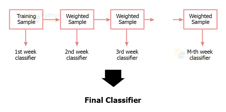
Unlike bagging, boosting does not aggregate the results of all its constituent learners. Instead, it arranges the trees in a sequential manner such that each consequent tree tries to eliminate the drawbacks of its previous trees. Each tree in this sequence tends to learn from its preceding tree and tries to update the residual error. As a result of which, trees that are next in sequence will have to deal with the updated version of the residual error.

We create the base learners for the boosting method in such a way, that they have a high bias and their predictive power is just a bit better than that of random guessing. These learners are weak learners and each of them contributes some vital information to the overall prediction results. This makes boosting an effective method since it generates a strong learner by combining the predictive power of the weak learners. As a result of which, we get a strong learner at the end, that has low bias as well as low variance.

What Algorithm does XGBoost Use?

We can implement the XGboost library using the gradient decision tree algorithm. This algorithm is quite extensively used and is known by many names like gradient boosting, multiple additive regression trees, stochastic gradient, and gradient boosting machines.

The main focus of this algorithm is that the consequent models tend to reduce the residual errors of their preceding trees and try to create a better model than the existing one. We keep on adding the models to the sequence till we observe no further improvement. The most popular example of this algorithm is the AdaBoost algorithm that predicts the output for data points for which prediction is quite difficult.

The gradient boosting is a very effective technique where the newly created models show a low variance and have a very precise predictive power since they try to rectify the error of the preceding trees in the sequence. The algorithm is called gradient boosting because it makes use of a gradient descent algorithm to reduce the errors and minimize the loss while adding the new trees to the sequence.

The strong point of this algorithm is that it is effective for both classification and regression predictive models.

Steps for XGBoost Installation

For installing XGBoost on the Windows Operating System, we need to follow either of the two approaches:

1. If we do not have git:

git clone –recursive https://github.com/dmlc/xgboost

2. If we do have git connectivity

git submodule init

git submodule update

In the case of OSX(Mac), we need to follow the steps as

brew install gcc@8

Features of XGBoost

The main focus of the technique is to make the model increase its computational power and the model to have a better performance. Apart from these, the technique offers more advanced features like:

1. Model Features

The model supports the various features of Scikit-learn and R implementations, along with new additions like regularization. The model supports these three forms of gradient boosting:

• Gradient Boosting Algorithm including learning rate.
• Stochastic Gradient Boosting with sub-sampling at column, row, and column per splits levels.
• Regularized Gradient Boosting with L1 as well as L2 regularization. This allows the algorithm to avoid overfitting.

2. System Features

The library delivers a system that is used in a range of computing environments like:

• Parallelization of tree construction using CPU cores during training.
• Distributed Computing for training large models.
• Out-of-Core computing for a huge dataset that we can’t fit in the main memory.
• Cache optimization for data structures and algorithms. XGBoost optimizes the use of hardware resources for non-contiguous memory access to get gradient statistics by row index. The technique achieves this by allocating internal buffers at each thread.

3. Algorithm Features

The developers implemented the algorithm in such a way that it facilitates the efficiency of the computing time and memory resources. The main goal of the algorithm development was to train the data in the best possible way with the available resources. Some key features of the algorithm implementation are:

• Sparse Aware implementation with the automated handling of missing data values. XGBoost incorporates a sparsity-aware split finding algorithm so that it can handle various sparsity patterns.
• Block Structure to support the parallelization of the tree sequence. This allows the technique to ensure that the computing speed is high by making use of multiple cores on the CPU. This technique bifurcates the data into in-memory units called blocks. This helps the technique to enable data layout by subsequent iteration.
• Continuous Training to ensure the further scope of development in an already fitted model.

Apart from these, it also provides features like:

4. Weighted Quantile Sketch

As we have seen earlier, most of the existing tree-based algorithms can find the split points when the dataset has data points of equal weights. But the algorithms are not well trained to efficiently handle weighted data. However, XGBoost is a distributed weighted quantile sketch algorithm and it effectively handles weighted data.

5. Block structure for parallel learning

For faster computing, XGBoost can make use of multiple cores on the CPU. This is possible because of a block structure in its system design. Data is sorted and stored in in-memory units called blocks. Unlike other algorithms, this enables the data layout to be reused by subsequent iterations, instead of computing it again.

6. Cache Awareness

In XGBoost, non-continuous memory access is required to get the gradient statistics by row index. Hence, XGBoost has been designed to make optimal use of hardware.

Implementation of XGBoost in Python

# PythonGeeks code for XGBoost classifier
# Importing the libraries
import numpy as np
import matplotlib.pyplot as plt
import pandas as pd
 
# Importing the dataset
dataset = pd.read_csv('Churn_Modelling.csv')
X = dataset.iloc[:, 3:13].values
y = dataset.iloc[:, 13].values
 
# Encoding categorical data
from sklearn.preprocessing import LabelEncoder, OneHotEncoder
labelencoder_X_1 = LabelEncoder()
 
X[:, 1] = labelencoder_X_1.fit_transform(X[:, 1])
labelencoder_X_2 = LabelEncoder()
 
X[:, 2] = labelencoder_X_2.fit_transform(X[:, 2])
onehotencoder = OneHotEncoder(categorical_features = [1])
 
X = onehotencoder.fit_transform(X).toarray()
X = X[:, 1:]
 
# Splitting the dataset into the Training set and Test set
from sklearn.model_selection import train_test_split
X_train, X_test, y_train, y_test = train_test_split(
    X, y, test_size = 0.2, random_state = 0)
 
# Fitting XGBoost to the training data
import xgboost as xgb
my_model = xgb.XGBClassifier()
my_model.fit(X_train, y_train)
 
# Predicting the Test set results
y_pred = my_model.predict(X_test)
 
# Making the Confusion Matrix
from sklearn.metrics import confusion_matrix
cm = confusion_matrix(y_test, y_pred)

The output of the above code will depict the following results

Accuracy will be about 0.8645

Reasons to Choose XGBoost

The two main factors to choose XGBoost over other algorithms are:

• Execution Speed
• Model Performance

Let us look at these points in brief

1. XGBoost Execution Speed

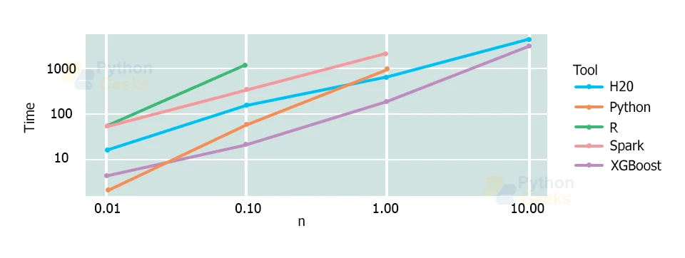
Usually, XGBoost exhibits really fast performance. When we compare the computational speed of XGBoost to other algorithms, it shows high variance in the speed of all other algorithms. Szilard Palka conducted an experiment to compare the performance of all the implementations of gradient boosting and the results are quite significant.

The results in the above graph demonstrate that XGBoost always shows a better performance rate as compared to other implementations from R, Python, Spark, and H2O.

2. XGBoost Model Performance

The main advantage of choosing XGBoost over other implementations is that it dominates the structures or tabular datasets on classification and regression predictive models.

The fact that it is amongst one of the go-to algorithms for the competition winners of the Kaggle competitive data science platform, gives testament to the efficiency of this algorithm.

3. Flexibility

XGBoosting enables user-defined objective functions with classification, regression, and ranking problems. We can even make use of an objective function to measure the performance of the model.

4. Availability

Because of its availability for programming languages such as R, Python, Java, Julia, and Scala, the language is quite extensive.

Conclusion

With this, we have reached the end of the article about the XGBoost method. We covered the basics of the XGBoost algorithm, along with the various features and pre-requisites of the model. We also saw some of the major features to choose XGBoost over other implementations. Hope that this PythonGeeks article was able to solve your queries regarding the XGBoost algorithm.