XGBoost Algorithm in Machine Learning

In the previous article, we saw the introduction of the XGBoost. We saw the various features of the algorithm and the reasons why we should use the algorithm over other implementations of gradient boosting algorithms. In this article, we will take our discussion of XGBoost further ahead and look at the implementation of the algorithm with Python.

Further, we will discuss the Advanced functionality of the XGBoost algorithm along with General Parametres, Booster Parameters, and Linear Booster Specific Parameters. Towards the end of the article, we will look at the reasons why we consider this algorithm superior. So, let’s dive straight into the article and try to know more about the XGBoost technique.

Introduction to XGBoost

In the last article, we saw a brief introduction to the XGBoost algorithm. As we have seen earlier, XGBoost is the implementation of the gradient descent decision tree structure used for classification as well as regression problems. The main aim behind the development of XGBoost was to improve the speed and performance of the training models.

XGboost is a type of software library that is mainly supported by the majority of the interfaces. Some of the interfaces that support the implementation of XGBoost are:

• C++, Java, and other JVM languages
• Julia
• CLI or Command Line Interface
• Python along with Scikit-learn
• R interface

Implementation of XGBoost using Python

Let us quickly look at the code to understand the working of XGBoost using the Python Interface.

Code:

As we know, Python has some pre-defined datasets for our users to make it simple for implementation. In this example, we are using the Boston housing dataset. Like any other dataset, we have to first import the set using the following command.

from sklearn.datasets import load_boston
boston = load_boston()
print(boston.keys())

Since the dataset of the Boston Housing acts like a Dictionary, we can use the .keys() method to access the dataset keys.

The output of the above code for the housing data set will be:

dict_keys([‘data’, ‘target’, ‘feature_names’, ‘DESCR’, ‘filename’, ‘data_module’])

You can easily check the shape of the dataset with the boston.data.shape() attribute.

print(boston.data.shape)

Resulting in the output

(506, 13)

The above output demonstrates that the dataset has 506 rows of data with 13 columns. Now to find out the names of these 13 columns, we can use the .feature_names attribute.

print(boston.feature_names)

The output of the above code for the features names is

#output[‘ZN’ ‘INDUS’ ‘CHAS’ ‘NOX’ ‘RM’ ‘AGE’ ‘DIS’ ‘RAD’ ‘TAX’ ‘PTRATIO’ ‘B’ ‘LSTAT’#names of the columns in the dataset

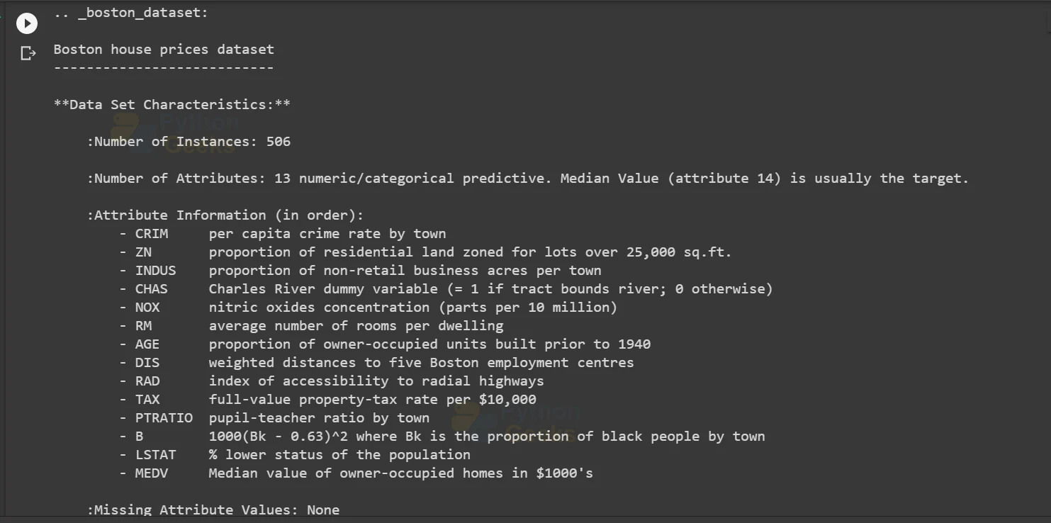
However, if you are not satisfied with knowing only the names of the columns of the dataset, then the description for the dataset is present in the dataset itself. We can use the .DESCR to show the description of our dataset.

print(boston.DESCR)

The result of the description attribute is

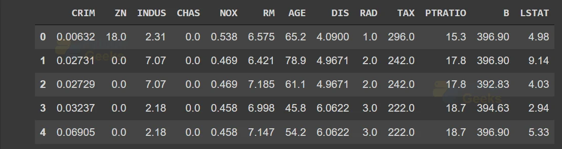
Now let’s convert this dataset into a Pandas data frame containing a series of information. For that we need to import the pandas library and call the DataFrame() function. We can observe the top 5 series of the dataframe using the .head() method.

import pandas as pd

data = pd.DataFrame(boston.data)
data.columns = boston.feature_names
data.head()

This will result in the following output for the housing dataset

Now that we know some of the basic functionalities of the dataset and the pandas data frame, let us look at the XGBoost implementation.

In the following code, we are about to build an XGBoost training model with trees as the base learners. We will use XGBoost’s Scikit-learn compatible API. Apart from this, we will also look at some of the tuning parameters that XGBoost uses to improve the performance of the model. Let us look at the full code in detail.

#PythonGeeks code for the implementation of XGBoost algorithm

#importing the necessary libraries
from sklearn.datasets import load_boston
#you can install python libraries like xgboost on your system using pip install xgboost on cmd
import xgboost as xgb
from sklearn.metrics import mean_squared_error
import pandas as pd
import numpy as np
import matplotlib.pyplot as plt

#loading the Boston Housing Dataset

boston = load_boston()

#converting the data into pandas dataframe using the DataFrame attribute

data = pd.DataFrame(boston.data)
data.columns = boston.feature_names

# we have to #Separate the target variable and rest of the variables using .iloc to subset the data.
X, y = data.iloc[:,:-1],data.iloc[:,-1]

# we will convert the dataset into an optimized data structure called Dmatrix that XGBoost supports
data_dmatrix = xgb.DMatrix(data=X,label=y)
from sklearn.model_selection import train_test_split

X_train, X_test, y_train, y_test = train_test_split(X, y, test_size=0.2, random_state=123)#For splitting the test data

# we have to #instantiate an XGBoost regressor object by calling the XGBRegressor() class from
#the XGBoost library with the hyper-parameters passed as arguments.
xg_reg = xgb.XGBRegressor(objective ='reg:linear', colsample_bytree = 0.3, learning_rate = 0.1,#for training data
max_depth = 5, alpha = 10, n_estimators = 10)#setting the parameters

#Fit the regressor to the training set and make predictions on the test set using the familiar .fit() and .predict() methods
xg_reg.fit(X_train,y_train)
preds = xg_reg.predict(X_test)

# we have to #Compute the rmse by invoking the mean_sqaured_error function from sklearn's
#metrics module.
rmse = np.sqrt(mean_squared_error(y_test, preds))
print("RMSE: %f" % (rmse))

#invoking XGBoost's cv() method and store the results in a cv_results DataFrame
params = {"objective":"reg:linear",'colsample_bytree': 0.3,'learning_rate': 0.1,
'max_depth': 5, 'alpha': 10}

cv_results = xgb.cv(dtrain=data_dmatrix, params=params, nfold=3,
num_boost_round=50,early_stopping_rounds=10,metrics="rmse", as_pandas=True, seed=123)

# we have to Extract and print the final boosting round metric.
print((cv_results["test-rmse-mean"]).tail(1))

#visualize individual trees from the fully boosted model
xg_reg = xgb.train(params=params, dtrain=data_dmatrix, num_boost_round=10)

xgb.plot_tree(xg_reg,num_trees=0)
plt.rcParams['figure.figsize'] = [50, 10]
plt.show()

The output of the following XGBoost code will be

Let us look at some of the parameters that we use while implementing XGBoost.

Parameters in XGBoost Algorithm

1. General Parameters

XGBoost has the following list of general parameters for the development of the model.

a. silent: this parameter retains its default values as 0 and we need to explicitly specify the value 1 for silent mode while 0 is used for printing running messages.

b. booster: we use this parameter to specify the value of the booster. It has gbtree as the default value which is used for tree-based booster and other is gblinear for linear function.

c. num_pbuffer: we do not need to explicitly set the value for this parameter since the XGBoost algorithm automatically sets the value for this parameter.

d. num_feature: like num_pbuffer, the XGBoost algorithm automatically sets the value for this parameter and we do not need to explicitly set the value for this.

2. Booster Parameters

As we know, XGBooster deals with tree-specific parameters that we are going to discuss below.

a. eta: the parameter attains the default value of 0.3 but we need to specify the step size shrinkage in an attempt to avoid overfitting. After the algorithm proceeds to each boosting step, we can automatically get the value of the weights of the new features. The main aim of eta is to shrink the feature weights that is consequently making the boosting process more conservative. Though the value for eta ranges from 0 to 1, a lower eta will indicate a model that is robust to overfitting.

b. gamma: the gamma parameter attains 0 as its default value while we need to specify the minimum loss reduction to make further participation on any leaf node. A larger value of gamma will indicate a more conservative algorithm. The range of values this parameter can attain is 0 to infinite.

c. max_depth: the parameter attains the default value as 6 while you have to specify the maximum depth of the tree. The range of values for the parameter ranges from 0 to infinite.

d. min_child_weight: the parameter attains the default values as 1 while you need to specify the minimum sum of instances of weights for a child. If the tree partition step will result in a leaf node, then the sum of weights is less than the min_child_weight. The parameter range value is from 0 to infinite.

e. max_delta_step: the parameter attains the default value as 0 and the max_delta_step will allow the tree’s weight estimation. The default value 0 states that the tree is set to no constraints. If we set the parameter with a positive value, then the update step becomes more conservative. The ideal values for this parameter range from 1 to 10 to obtain better results. The range of values for this parameter is from 0 to infinite.

f. subsample: the parameter attains the default value as 1 while we need to specify the subsample ratio of the training instance. As an example, if the value of this parameter is set to 0.5, then it means that the algorithm has chosen half of the data instances. The range of values for the subsample parameter is from 0 to 1.

g. cosample_bytree: the parameter attains the default value as 1 while we need to set the subsample ratio of columns when constructing trees for the model. The range of values for the cosample_bytree parameter is from 0 to 1.

3. Linear Booster Specific Parameters

The Linear Booster Specific Parameters in the XGBoost algorithm are:

a. lambda and alpha: these are the regularization terms for the weights of the leaf. While lambda attains 1 as its default value, alpha attains the default as 0.

b. lambda_bias: it is an L2 regularization term on the bias with the default value of 0.

4. Learning Task Parameters

The Learning Task Parameters of the XGBoost algorithm are:

a. base_score: the parameter attains the default value as 0.5 while we need to specify the initial prediction score of all the instances including global bias.

b. objective: the default value of the parameter is reg:linear while we need to specify the type of learner that we want for the algorithm. This includes linear regression, Poisson regression, and so on.

c. eval_metric: we need to specify the evaluation of the metrics for data validation. Then the algorithm will assign a default metric to the objective.

d. seed: for this parameter, we need to specify the seed to reproduce the same set of outputs.

Power of XGBoost Algorithm

The main characteristic of this algorithm that sets it apart from the other gradient descent implementations is its scalability. It offers a fast-learning model through parallel and distributed computing which in turn results in efficient memory management.

As a matter of fact, CERN recognizes this algorithm as the best approach to classify signals from the Large Hadron Collider for its performance. In this challenge by CERN, the algorithms needed to have a scalability factor to process the data that was generated at the rate of 3 petabytes per year. It also required the models to effectively distinguish an extremely rare signal from background noises in a complex physical process. Amongst all the competing algorithms, XGBoost was the most efficient and scalable solution for the robust model.

Conclusion

With that, we have reached the end of this article that talks about the XGBoost Algorithm in further detail. We came across the implementation of XGBoost in Python. We walked through a detailed introduction of the various parameters that we use in the implementation of XGBoost. Lastly, we came to know about the power of this algorithm in comparison to the other algorithms. In conclusion to this article, we can only say that XGBoost is certainly proving to be a game-changer in the field of classification and regression algorithms.