Commonly Used Machine Learning Algorithms

Till now, you must have heard enough about the various merits of Machine Learning. How it helps major companies in customizing their results according to their users, how machine learning reduces human interference and thus reduces the possibilities of errors. You even came across the topic of how Machine Learning algorithms would take over future technology. You even became familiar with the top tools to implement all the Machine Learning algorithms.

But the real question that would pester you now would be, how are you going to perform all the complex tasks that we’ve discussed so far? How will you fabricate the code in such a way that the system would automate itself and reduce your interference? Well, this article from PythonGeeks is here to facilitate all your queries.

As we know, every extensive result is an outcome of trivial fundamentals. And for Machine Learning, these trivial fundamentals are algorithms. In the general term, an algorithm is a set of steps that you need to perform in order to get your anticipated outcome. The complex Machine Learning codes are written with the help of simple algorithms. This PythonGeeks article would guide you on the basics of the top algorithms used for Machine Learning codes and how they are classified. So, let’s get on board and see the classification of the Machine Learning algorithms

Classification of Machine Learning Algorithms

In order to categorize the algorithms, they are broadly classified into two main categories, namely, Supervised Learning, Unsupervised Learning. Grouping these algorithms in such broad categories will help us to understand them better and help us in employing them properly. These categories are explained in detail below:

Supervised Learning

As the name suggests, Supervised Learning has the presence of a supervisor or an instructor. Algorithms classified under this type of learning deal with “labeled data”. By labeled data, we mean the data that has already been tagged to the correct answer. Now, you can use this trained dataset as an instructor to predict the correct output for the new set of input data. This type of learning basically maps the variable input with the correct output on the basis of the trained data.

Supervised Learning is again divided into two types on the basis of the problem faced. You can classify these types as Classification and Regression.

Unsupervised Learning

In Supervised Learning, we understood that you can train models using labeled data to predict the output. But every dataset doesn’t have labeled sets and, in such cases, we have to look for hidden patterns in the datasets. As the name suggests unsupervised learning algorithms do not require any instructor to guide the output. As opposed to supervised learning, these algorithms train the models in such a way that the models themselves find the patterns and insights hidden in the input dataset.

Like Supervised Learning, you can also classify Unsupervised Learning into two types depending on the type of problem encountered, namely, Clustering and Association.

Now that we know we know the broad classifications of the algorithms, we’ll look at the 9 most used algorithms for Machine Learning.

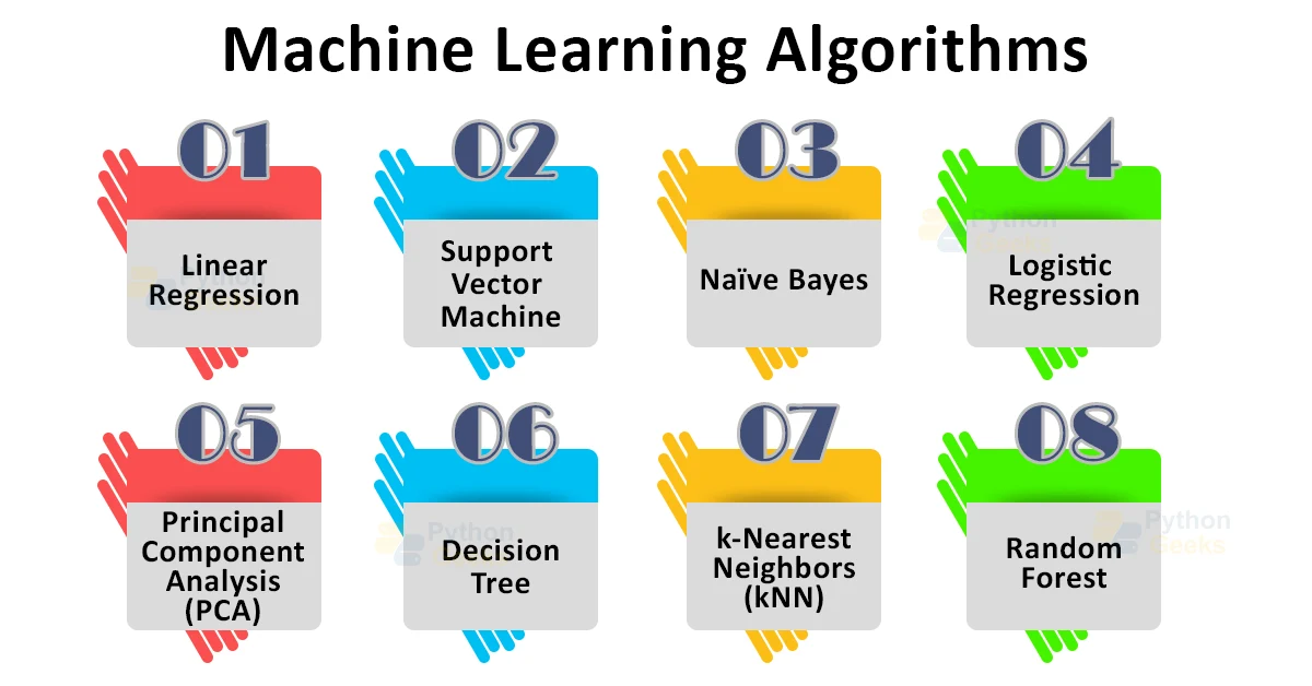
1. Linear Regression

This algorithm emanates under the Supervised Learning algorithm and tends to map the relationship between continuous target variables and one or more independent variables. As the name suggests, this algorithm tries to fabricate a linear relationship with the dependent and independent variables. There are various tools like scatter plots or correlation matrix, by means of which we can correlate the data in linear relationships.

A linear regression model tends to adapt a regression line to the scattered data points that represent the correlation accurately. The most common technique used to achieve this is ordinary-least squares (OLE). In this method, the model tends to find the best regression line by minimizing the sum of squares of the distance between data points and the regression line.

2. Support Vector Machine

This algorithm is a Supervised Learning algorithm and is generally used for the classification of the labeled data but you can also use it for regression problems.

The most critical part of implementing this algorithm is determining and representing a decision boundary. The decision Boundary is a line plotted on the regression graph to distinguish the various classes. Before determining the decision boundary, you have to plot each data point or each observation in n-dimensional space, where n is the number of distinguished features.

For example, if our sample dataset has the features “length” and “width” as the distinguishing features, then you have to create the plots for a 2-dimensional space and the decision boundary can be thought of as a line. Similarly, if our dataset has 3 distinguishing features, then the plot will have a 3-dimensional space and the decision boundary will be a plane in the space.

Furthermore, draw the boundary in such a way that the distance from the data points to the support vectors is maximum. In a possible condition, if the decision boundary is too close to support the vector, then it will be highly sensitive and you won’t be able to generalize.

In case the data points scatter too much, then drawing a stable boundary isn’t possible. When such is the case, the SVM uses a kernel trick that measures the closeness in the features of the points to develop a linear relationship between them.

SVM is very useful for the datasets in which the distinguishing features or the plot dimensions are comparably more than the cases in the dataset. But for large databases, the training time which adversely affects the algorithm performance.

3. Naïve Bayes

Naïve Bayes is again an example of Supervised Learning which is used for classification problems; therefore, it is sometimes referred to as Naïve Bayes Classification.

This algorithm assumes that the provided dataset would have features that are in no way similar to each other. In real world problems, finding such datasets which do not have any common features is hard to find. This naïve assumption of the algorithm is what gives the algorithm the name as “naïve”.

The main principle behind the Naïve Bayes algorithm is the Bayes Theorem

p(A|B) = p(A).p(B|A)p(B)

We need an extensively large dataset to apply the Naïve Bayes algorithm, to distinguish the various features of the data points. To avoid these anomalies, the algorithm assumes that all features are not correlated.

Here, the algorithm uses the concept of conditional probability for a single feature given the class labels are different. Here, the assumption that all the features are not correlated makes this algorithm fast compared to the other algorithms. But this also makes the algorithm less accurate since it’ll not consider all the data points. So, if your problem deals more with speed than accuracy, the Naive Bayes algorithm will be the best-suited option for you.

4. Logistic Regression

Logistic Regression is a Supervised Learning algorithm that is used for classification problems. Though the name of the algorithm may seem to classify it as a regression algorithm, it is the word logistic; which refers to a logical function that performs the classification task. Logistic regression is a powerful algorithm when it comes to dealing with problems like spam email separation, ad click prediction and customer churn.

The fundamentals of this algorithm lie in the logistic function also known as the sigmoid function. This function takes the data points as input and tends to map them to any real number values between 1 and 0. You can write the sigmoid equation as:

y=11+ⅇ-x

The logistic regression algorithm takes a linear equation as the input and passes it through the sigmoid function to perform the binary classification.

The values of the output tend to be positive or negative. A positive value ascertains a sure incident. Since, we are not always sure whether to classify the email as spam or not, we never tend to classify it as spam unless we are almost sure of it. So, the values that lie between the threshold of positives and negatives, tends to be a problematic area for this algorithm.

5. Principal Component Analysis (PCA)

PCA is a dimensionality reduction algorithm. In simpler words, it tends to create new features of the given datasets from the existing ones, by keeping much of the information as it is. It occurs under unsupervised learning, but it is extensively used as a pre-processing stage for supervised learning algorithms.

The main focus of this algorithm is to find a new feature for the dataset by grouping together the existing features on the basis of their commonalities. These newly derived features are what we call Principal Components. You have to decide the order of these components on the basis of their variation from the previous features from which you derive them.

The main advantage of using PCA is that a much extensive amount of the original dataset variance is preserved as well as the number of features of the dataset is reduced significantly.

6. Decision Tree

The basic idea behind the implementation of the decision tree is the portioning of the dataset. The algorithm recursively asks questions to the dataset for its processing. The first major split is based upon a common property and the dataset is then repeatedly classified by asking similar questions to each individual classified component.

The major focus of the decision tree is to exponentially increase the predictiveness at each portioning point. This helps the model to gain more clarity about the dataset. Thus, you cannot randomly split data at any given partition. Parting the data at such a point where the data becomes more accessible proves beneficial for the algorithm.

Now, the question here is, how long do you need to keep asking the question? When will our data tree become sufficient enough to answer its own queries? Well, the answer is quite simple. The model can keep asking the questions until all the nodes become pure. The previously trained data can give the results with high accuracy but the newly trained model can yield less accurate results.

7. k-Nearest Neighbors (kNN)

KNN is a supervised algorithm that is adequate in solving both classification and regression problems. The main idea behind the algorithm is that it uses the neighbors of the data points to predict the value of the concerned data point.

The algorithm checks the neighboring points of the class of the data to find its value. For example, if you take it to be 8, then the algorithm would consider 8 neighboring items to evaluate the value of the given data point.

The value of k determines the accuracy of the algorithm. In other words, the lesser the value of k, the more generalized is the behavior of the model. Thus, we are likely to end up with an overfit model for the problem. On the other hand, if the value of k is too high, then the model would be too generalized and won’t be of any use for prediction of the output.

The major advantage of using kNN is that it does not involve any assumptions and is too easy to interpret. The data points required in this algorithm aren’t high, which is memory efficient.

8. Random Forest

A collaborative group of decision trees is what we refer to as a Random Forest. You can efficiently use Random forest as it is a highly accurate model for many diverse problems and does not require normalization or scaling. However, it is not beneficial for high-dimensional data sets as compared to other quicker linear models.

If you use random forest for a classification problem, then the result is based on the majority vote of the results received from individual decision trees. For the regression model, the prediction of a leaf node is the mean value of the target values in that particular leaf. The random forest regression model takes the mean value of the results from each decision tree for accuracy.

Random forest models reduce the possibilities of overfitting and hence accuracy is much higher as compared to a single decision tree. Furthermore, you have to operate decision trees in a random forest in parallel summation so that you don’t have to face the hindrance due to time.

9. Gradient Boosted Decision Tree (GBDT)

Like Random Forest, GBDT is also an ensemble algorithm that makes use of the boosting method to combine individual decision trees for accuracy over an individual decision tree.

The key difference between Random Forest and GBDT is the use of boosting. Boosting refers to combining a learning algorithm in series to achieve a resilient learner from numerous consecutively connected weak learners.
In the above context, weak learners refer to decision trees.

In order to enhance accuracy, each decision tree in the GBDT attempts to minimize the errors of the previous tree. Trees in boosting are weak links. However, adding numerous such trees in series where each tree focuses on the errors of the previous one, this is what makes boosting a highly proficient and accurate model. Unlike bagging, boosting does not encompass bootstrap sampling. Everytime you add a new tree to the model, it is added to a modified version of the preliminary dataset.

GBDT is a very useful model for both classification and regression Problems. It is a much more accurate model as compared to random forests. It is also able to handle mixed types of features for which no preprocessing is needed. You need to carefully tune the hyperparameters in order to avert the model from overfitting.

10. k-Means Clustering

K-means clustering tends to group the data on the basis of similarities. It groups the data points in such a way that the points sharing similar properties lie in the same group and those with dissimilarities are grouped separately. You can find out the similarities between the points by observing the distance between them.

The groups are at such a distance, that the distance between similar points is minimized and the distance between dissimilar points is maximized. However, you can not predict the number of clusters that are formed. The challenging task thus becomes to accurately specify the number of clustering groups prior to modeling. The challenge becomes much more complex since the data in the real world is much more complex and difficult to group.

After determining the number of clusters in advance, the algorithm is performed in the following steps:

• You need to randomly select a centroid for each cluster.
• Now you’ve to determine the distance between each data point from the centroid.
• Data Points are now assigned to the closest cluster to them.
• You’ll now have to calculate the mean of all the data points in the cluster and determine the new centroid.
• Now, recursively perform the above steps until you cover all the points so that the center of the data points stops moving.

11. DBSCAN Clustering

DBSCAN stands for Density-Based Spatial Clustering of Applications with Noise, which is another form of clustering algorithm. As the name suggests, this algorithm deals with datasets that have cluster density. Previously studied algorithms like k-means clustering and hierarchical clustering are not effective when it comes to datasets that have arbitrary shape.

The main principle behind this algorithm is, a point is said to be a part of the cluster if it is close to the maximum number of points of the cluster.

The algorithm deals with two major parameters, namely, eps and minPts. While eps demonstrate the shortest distance for the points to be considered as neighbors, minPts determines the minimum number of points required to form a cluster.

Based on these parameters, the data points are categorized in three groups, namely, core points (points that have minimum number of minPts in the given eps), border point (points that are reachable from the core points) and outliers (points that are neither core nor border).

The major advantage of DBSCAN over partitioned-based clustering is that you do not have to determine the number
of clusters in advance. However, the major difficulty may lie in determining the eps.

Conclusion

In this way, you’ve studied in brief about the various algorithms that constitute the Machine Learning models. Consecutively, you’ll now be able to apply these algorithms according to your problems. You can now train and deploy efficient and fully-functioning models which would enhance the domain of Machine Learning.