Support Vector Machine
Get Ready for Your Dream Job: Click, Learn, Succeed, Start Now!
As we have seen in the earlier tutorials, Classification problems come under the Supervised Learning algorithm. Therefore, PythonGeeks brings to you an article that will brief you on the algorithm that deals with the classification problem- Support Vector Machine(SVM). So, let us start by understanding the basics of SVM.
Introduction to Support Vector Machine
As we have seen in the earlier articles, a Support Vector Machine is a type of Supervised Machine Learning algorithm. Though it is capable of handling both regressions along with classification problems, it is predominantly used in classification problems.
The main focus of this algorithm is to locate a hyperplane in an N-dimensional space that will classify the different data points. The hyperplane in this discussion is the decision boundary that will segregate the data points based on their features. This will help the algorithm to place the new data points in the classified area. The number of features of the data points determines the dimension of the hyperplane.
As an example, if we consider a dataset with 2 distinct data point features, then the hyperplane for this dataset will be a line.
There are two types of Support Vector Machines are:
1. Linear SVM: This type of SVM is useful when we have to deal with data that has exactly two distinguishing features for the data points. Here, the hyperplane for the dataset will be a straight line. Such a dataset that is separated by a line is linearly separable data. The classification technique we use for this type of data is Linear SVM.
2. Non-Linear SVM: Unlike Linear SVM, Non-linear SVM takes charge of the classification of the data points when the dataset is not linearly separable. This means that non-linear SVM works on data sets that we cannot separate with a straight line.
Now that we know the basics of SVM, let us look at the working of SVM
Kernel in SVM
In a practical sense, we implement the SVM algorithm with the kernel that transforms an input data space into the required form. SVM makes use of a technique called the kernel trick in which the kernel takes the input as a low dimensional space and transforms it into a higher-dimensional space. In other words, the kernel converts non-separable problems into separable problems with the addition of more dimensions to it. It makes SVM more powerful, flexible, and precise. We will now discuss the types of kernels used by SVM.
1. Linear Kernel Function
This is the most basic type of kernel that we use for SVM classification. It is a one-dimensional kernel. The mathematical representation is
K (xi, xj) = xi. xj +c
2. Polynomial Kernel Function
This type of kernel is mostly used for image processing algorithms. It is a general representation of the kernels having degree more than one.
The polynomial kernel is further divided into two types:
a. Homogeneous Polynomial Kernel
K(xi, xj) = (xi . xj)d
In this function, we take the dot product of both the numbers and d represents the degree of the polynomial.
b. Inhomogeneous Polynomial Kernel
K (xi, xj) = (xi . xj + c)d here c is a constant
3. Gaussian RBF Kernel
RBL is the acronym for Radial Basis Function. We prefer this kernel function when we do not have any prior knowledge of the data.
K (xi, xj) = exp(-ϒ||xi – xj||)2
Working of Support Vector Machine
1. Working for linear SVM
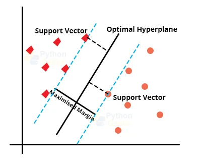
To understand the working of SVM in a comprehensive and easy way, let us consider an example of a data set having two distinguishing features, let us consider them to be the colors blue and green. Now, we want to add two new data points, namely x1 and x2 to this existing data set and classify them under the features blue and green. As the dataset has 2 features, we will represent the data points in a 2-dimensional plane whose hyperplane will be a straight line.

As we can observe in the image below, the two classes of data can be separated using multiple straight lines. However, SVM tends to look for the best possible solution to classify the points in the given plane. The best possible decision boundary for this dataset will emerge as the hyperplane of the dataset. The algorithm tends to locate the classes at a minimum distance from the points present on it. These points on the line are called support vectors.
The distance that spans between the support vectors and the hyperplane is the margin. The best possible line that will minimize this margin is the optimal hyperplane for the given dataset.
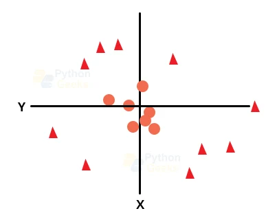
2. Working for non-linear SVM
As we have seen in the earlier example, if we have a linearly separable dataset, then we can easily segregate the different classes using a straight line. However, if we do not have linearly separable data, then we cannot segregate the classes using a straight line. In order to segregate these data points, we need to add one more dimension to the dataset. In the linear dataset, we had dimensions x and y.
To handle non-linear data, we will add one more dimension z to it, where z=x2+y2. By doing so, our sample space will look like the image below.
Therefore, we now need to deal with a 3-dimensional dataset whose hyperplane will be a 2-dimensional shape. We can look at the hyperplane of the non-linear dataset as below.

Now that we know the working of both linear and non-linear SVM, let us look at the implementation of SVM using Python.
Implementation of SVM using Python
Code for the SVM implementation
# PythonGeeks Code for the implementation of SVM
#Importing the necessary libraries
import pandas as pd
import numpy as np
import matplotlib.pyplot as plt
from matplotlib.colors import ListedColormap
import matplotlib.pyplot as plt
from sklearn import datasets
from sklearn.svm import SVC
from sklearn.model_selection import train_test_split
from sklearn.preprocessing import StandardScaler
%pylab inline
#we will use the iris dataset that is available with the load_iris() method.
pylab.rcParams['figure.figsize'] = (10, 6)
iris_data = datasets.load_iris()
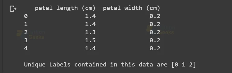
# We'll use the petal length and width only for this analysis
X = iris_data.data[:, [2, 3]]
y = iris_data.target
# Input the iris data into the pandas dataframe
iris_dataframe = pd.DataFrame(iris_data.data[:, [2, 3]],
columns=iris_data.feature_names[2:])
# View the first 5 rows of the data
print(iris_dataframe.head())
# Print the unique labels of the dataset
print('\n' + 'Unique Labels contained in this data are '
+ str(np.unique(y)))
The output of the above code results in
#we will split our data into training and test set using the train_test_split() function
X_train, X_test, y_train, y_test = train_test_split(X, y, test_size=0.3, random_state=0)

print('The training set contains {} samples and the test set contains {} samples'.format(X_train.shape[0], X_test.shape[0]))
markers = ('x', 's', 'o')
colors = ('red', 'blue', 'green')
cmap = ListedColormap(colors[:len(np.unique(y_test))])
for idx, cl in enumerate(np.unique(y)):
    plt.scatter(x=X[y == cl, 0], y=X[y == cl, 1],
           c=cmap(idx), marker=markers[idx], label=cl)
The above code outputs in the following way

standard_scaler = StandardScaler()
standard_scaler.fit(X_train)

X_train_standard = standard_scaler.transform(X_train)
X_test_standard = standard_scaler.transform(X_test)

print('The first five rows after standardisation look like this:\n')
print(pd.DataFrame(X_train_standard, columns=iris_dataframe.columns).head())
#PythonGeeks
SVM = SVC(kernel='rbf', random_state=0, gamma=.10, C=1.0)
SVM.fit(X_train_standard, y_train)

print('Accuracy of our SVM model on the training data is {:.2f} out of 1'.format(SVM.score(X_train_standard, y_train)))

print('Accuracy of our SVM model on the test data is {:.2f} out of 1'.format(SVM.score(X_test_standard, y_test)))
import warnings
def versiontuple(version):
   return tuple(map(int, (version.split("."))))
def decision_plot(X, y, classifier, test_idx=None, resolution=0.02):

   # setup marker generator and color map
   markers = ('s', 'x', 'o', '^', 'v')
   colors = ('red', 'blue', 'green', 'gray', 'cyan')
   cmap = ListedColormap(colors[:len(np.unique(y))])

   # plot the decision surface
   x1min, x1max = X[:, 0].min() - 1, X[:, 0].max() + 1
   x2min, x2max = X[:, 1].min() - 1, X[:, 1].max() + 1
   xx1, xx2 = np.meshgrid(np.arange(x1min, x1max, resolution),
                 np.arange(x2min, x2max, resolution))
   Z = classifier.predict(np.array([xx1.ravel(), xx2.ravel()]).T)
   Z = Z.reshape(xx1.shape)
   plt.contourf(xx1, xx2, Z, alpha=0.4, cmap=cmap)
   plt.xlim(xx1.min(), xx1.max())
   plt.ylim(xx2.min(), xx2.max())
   for idx, cl in enumerate(np.unique(y)):
      plt.scatter(x=X[y == cl, 0], y=X[y == cl, 1],
              alpha=0.8, c=cmap(idx),
              marker=markers[idx], label=cl)
      decision_plot(X_test_standard, y_test, SVM)
The output of the above code is

Now that we know how to implement SVM using the data science libraries of Python, let us look at the advantages and disadvantages of Python.
Advantages of SVM
1. Optimization: As we have seen in the working of SVM, the algorithm always tends to look for global minima instead of working with many local minima. This solution that we find using SVM will have a definiteness to it.
2. Implementation: Since SVM is a widely known algorithm, all the major Machine Learning Tools support the implementation of SVM. You can use anything from TensorFlow to Mahout to implement this algorithm.
3. As we have seen in the above sections, SVM is favorable for both linearly separable along with non-linearly separable datasets. This makes the accessibility of the algorithm to be quite extensible.
4. SVMs are used on both labeled as well as unlabeled data. It only requires the condition for segregation for the classification of the datasets.
5. Conventional classifications were computationally expensive when it came to dealing with feature mapping. However, with the help of SVMs, we can conveniently reduce the complexities of the feature mapping.
Disadvantages of SVM
1. SVMs are incapable of handling sequential datasets. This leads to the loss of crucial data points while dealing with text structures of the input data.
2. Developers prefer logistic regression over Vanilla SVM as the latter is incapable of providing probabilistic confidence. This gives logistic regression an upper hand over SVM in prediction problems.
3. As SVM supports a variety of kernels, it becomes quite troublesome when we have to deal with the choice of kernel. After considering the diversity in the options available for the kernel, it becomes quite hectic to decide on the best kernel.
Tuning SVM Parameters
1. Kernel
The kernel in SVM focuses on transforming the input data into the form that we require. Some of the examples of kernels that we use in SVM are linear, polynomial, and radial basis function (RBF). When we deal with a non-linearly separable dataset, we use RBF and Polynomial functions. When we deal with more complex data, we need to use more advanced kernels to segregate the classes. With the help of these kernels, we are able to have accurate classifiers.
2. Regularization
We are able to maintain regularization in the given dataset by adjusting it in the Scikit-learn’s C parameters. C, in this context, denotes a penalty parameter that represents an error or any form of misclassification. With this misclassification, we can understand how much of the error is bearable by the machine. With the help of this, we can nullify the compensation between the misclassified term and the hyperplane.
The smaller the value of the C parameter, the smaller will be the margin value for the hyperplane of the dataset. Similarly, a larger C value demonstrates larger margin values for the dataset.
3. Gamma
If we have a lower value of Gamma, it will create a loose fit of the training dataset. On the contrary, a high value of gamma will make the model fit in the set more accurately. A low gamma value only gives preference to the nearby points for the calculation of a separate plane. However, a higher value of gamma will consider all the data points for calculating the final separation line.
Applications of Support Vector Machine
Some of the major advantages of SVM are listed below.
1. Face Detection
As we know, SVM is a classification algorithm. We can conveniently apply this algorithm with other image processing algorithms to classify the images. We can even separate out distinguishing features from the image itself.
2. Text and Hypertext Categorization
SVM proves to be a handy algorithm when it comes to text and hypertext categorization. It is useful for the classification of the documents that we provide as input. It compares the score generated by the documents to the threshold value of the document.
3. Handwriting Recognition
SVM is a great tool for segregating the handwritings according to the provided input dataset. When we use it along with other image processing algorithms, it can accurately distinguish legal handwriting.
Conclusion
With that, we have reached the conclusion of this article. In the discussion, we tried to get a brief idea about the Support Vector Machine and its working. We also came across the concepts of kernel, and gamma. Apart from them, we saw the implementation of SVM using Python. Hope that this PythonGeeks article proved beneficial to solve your SVM queries.
