Python SciPy Tutorial for Beginners
Master Programming with Our Comprehensive Courses Enroll Now!
How many of you find mathematics the hardest subject? This is because it involves complex and time-consuming calculations. Do you know Python has modules that help us in doing these operations in a few lines of code? In this article, we will learn about Python library called SciPy and its different methods that can be used for different uses with examples. So, let us start with an introduction to this library.
Introduction to Python SciPy
SciPy is a free and open-source library in Python that is used for scientific and mathematical computations. It is pronounced as Sigh Pie. This is an extension of NumPy. It contains a wide range of algorithms and functions to do mathematical calculations, manipulating, and visualizing data.
The modules in this library allow us to do the below operations:
1. Linear algebra
2. Integration
3. Optimization
4. Interpolation
5. Special functions
6. Signal and Image processing
7. ODE solvers
Advantages of using Python SciPy
1. It is Open-source
2. It is easy to use and it is also fast.
3. Contains high-level commands and classes to do visualization and manipulation of data.
4. Also includes classes, and web and database routines that support parallel programming.
Installing and Importing SciPy
SciPy cannot be used directly by importing it as it does not get downloaded along with the IDE. So, we need to install it before using it.
There are different ways of installing modules in Python. Let us see each of them:
1. Installing Python SciPy using pip
Pip stands for ‘Pip Installs Packages’ and it can be used as a standard package manager. We can install it on any operating system. Using pip we can install SciPy using the below command.
pip install scipy
2. Installing SciPy using Anaconda
If we have the anaconda navigator downloaded we can use this to install Python SciPy by writing the below command.
conda install -c anaconda scipy
Done with the installation, we can now import the library by writing the below statement.
import scipy
Let us also import the NumPy and Matplotlib libraries which will be used further along with SciPy in Python.
import numpy
import matplotlib
Sub packages in Python SciPy
The SciPy library provides various modules or sub-packages that we can use for different applications. These are listed in the below table.
| S.No. | Sub-package Name | Description |
| 1. | cluster | These are used for cluster algorithms like vector quantization/ Kmeans. |
| 2. | constants | It contains physical and mathematical constants. |
| 3. | fftpack | It contains algorithms to compute Fourier transforms. |
| 4. | integrate | It is a routine to do integration |
| 5. | interpolation | It contains tools to do interpolation and smoothing splines |
| 6. | io | It contains input and output tools for data |
| 7. | lib | It is a wrapper to an external library |
| 8. | linalg | It contains routines for linear algebra |
| 9. | misc | It is used for miscellaneous tools for reading and writing image |
| 10. | ndimage | It is used for the multidimensional dimension image processing |
| 11. | odr | It is used for orthogonal distance regression. |
| 12. | optimize | It contains algorithms for optimization. |
| 13. | signal | It has tools used for signal processing. |
| 14. | sparse | It contains sparse matrices and related routines |
| 15. | spatial | It contains spatial data structures and algorithms. |
| 16. | special | It has special functions |
| 17. | stats | It has tools to do statistics |
| 18. | weave | It contains functions to write C++/C code in the form of multiline strings. |
To import these sub-packages we use the following syntax:
from scipy import subpackage_name
Let us discuss these sub-packages in the further sections.
Constants in SciPy
This package includes various constants that can be used for various scientific calculations purposes. Let us see some of these constants. The constants available mathematical calculations are:
| Constant | Description |
| pi | Holds the pi value |
| golden | Holds the value of the golden ratio |
The physics constants are:
| Constant | Description |
| c | Holds speed of light in vacuum |
| speed_of_light | Holds speed of light in vacuum |
| G | It is the value of the standard acceleration of gravity |
| G | It is the value of the newton Constant of gravitation |
| E | It holds the elementary charge |
| R | It represents the molar gas constant |
| Alpha | It is the value of fine-structure constant |
| N_A | It holds the value of Avogadro constant |
| K | It represents Boltzmann constant |
| Sigma | It is the value of the Stefan-Boltzmann constant σ |
| m_e | It is the mass of the electron |
| m_p | It is the mass of the proton |
| m_n | It is the mass of the neutron |
| H | It represents Plank Constant |
| Plank constant | This also represents Plank constant h |
SciPy also provides a function called find() that returns the keys of constants that c
SciPy also provides a function called find() that returns the keys of constants that contain the given string. The below code shows an example.
Example of finding constants:
from scipy.constants import find
find('newton')
Output:
‘Newtonian constant of gravitation over h-bar c’]
In addition, we can also use the help() function.
Linear Algebra Sub Package in SciPy
This subpackage helps us solve the problems related to linear equations and their representation using vector spaces and matrices. It is built on ATLAS (Automatically Tuned Linear Algebra Software), LAPACK(Linear Algebra Package), and BLAS(Basic Linear Algebra Subprograms) libraries. So, its computational speed is faster.
We can import this by writing
from scipy import linalg
Let us see some of the applications of linalg.
1. Solving a set of linear equations:
Let us say we want to solve two equations in x,y
2x+y=5
4y-5x=7.
Then we can solve it using the below code.
Example of solving a set of linear equations:
import numpy as np
from scipy import linalg

# Creating the input array
a = np.array([[2, 1], [4,-5]])
# Creating the solution Array
b = np.array([[5], [7]])

# Solve the linear algebra to find values of x and y that satisfy the equations
x = linalg.solve(a, b)

# Printing the results
print(x)

# Checking if the values are right by substituting them
print("\n Checking the results, the values must be zeros")
print(a.dot(x) - b)
Output:
[0.42857143]]
Checking the results, the values must be zeros
[[0.]
[0.]]
In this example,
a. We are first importing the required modules
b. Then we are creating the input array that stores the coefficients of the variables and the solution array that represents the constant value of the right-hand side of the equality symbol.
c. Then we used the solve() method to find the solutions of x,y
d. Then we checked the obtained results by substitution using the dot() function
We can see that the final outputs are zeros which shows that the obtained solution is correct.
2. Finding determinants of matrices
We can find the determinant first by creating the square matrix and then using the det() function. For example,
Example of finding the determinant of the matrix:
from scipy import linalg
import numpy as np

#Making the numpy array
mat = np.array([[1,2,3],[3,4,5],[7,8,6]])

#Passing the matrix  to the det function
x = linalg.det(mat)

#printing the determinant
print(f'Determinant of the matrix\n{mat} \n is {x}')
Output:
[[1 2 3]
[3 4 5]
[7 8 6]]
is 5.999999999999998
3. Finding the inverse of a matrix
Similar to the determinant function(), we can first create the matrix and use the inv() function. An example is shown below.
Example of finding the inverse of the matrix:
from scipy import linalg
import numpy as np

#Making the numpy array
mat = np.array([[1,1,1],[2,4,5],[3,4,3]])

#finding the inverse of the matrix using the inv() function
mat2 = linalg.inv(mat)

#printing the original and inverse matrices
print(f'Inverse of the matrix\n{mat} \n is \n{mat2}')
Output:
[[1 1 1]
[2 4 5]
[3 4 3]]
is
[[ 2.66666667 -0.33333333 -0.33333333]
[-3. 0. 1. ]
[ 1.33333333 0.33333333 -0.66666667]]
4. Singular value decomposition
We can find the decomposition of the matrix into a product of two orthonormal matrices and a diagonal matrix using the svd() function. For example,
Example of finding the svd of the matrix:
from scipy import linalg
import numpy as np

#Making the numpy array
mat = np.array([[1,4],[9,3]])

#printing the svd of the matrix
print(linalg.svd(mat))
Output:
[-0.96612059, 0.25809107]]), array([9.77803534, 3.3749111 ]), array([[-0.91564165, -0.40199548],
[ 0.40199548, -0.91564165]]))
5. LU decomposition
We can decompose the matrix into the product of lower and upper triangular matrices using the lu() function.
Example of finding the lu decomposition of the matrix:
from scipy import linalg
import numpy as np

#Making the numpy array
mat = np.array([[1,4],[9,3]])

#printing the lu decomposition of the matrix
print(linalg.lu(mat))
Output:
[1., 0.]]), array([[1. , 0. ],
[0.11111111, 1. ]]), array([[9. , 3. ],
[0. , 3.66666667]]))
6. Finding eigenvalues and eigenvectors
We can find the eigenvalues and the corresponding eigenvectors of the matrix using the eig() function. For example,
Example of finding the eigenvalues and the eigenvectors of the matrix:
from scipy import linalg
import numpy as np

#Making the numpy array
mat = np.array([[3,2,7],[1,3,0],[4,6,8]])

#Finding the eigenvalues and the eigenvectors
vals, vects = linalg.eig(mat)

#printing the eigenvalues
print("Eigenvalues:",vals)

#printing the eigenvectors
print("Eigen vectors:\n",vects)
Output:
Eigen vectors:
[[-0.63017668 -0.88721395 0.87240058]
[-0.07148854 0.44360698 -0.48064217]
[-0.77315376 0.12674485 -0.08888376]]
Polynomials in SciPy
We can solve the polynomial equations in SciPy using the poly1d module in NumPy. The below example shows different operations we can do.
Example of working on polynomials:
from numpy import poly1d

poly=poly1d([1,3,5]) #creating the polynomial
print("The polynomial is:\n",poly)

print("The value of the polynomial for the value of x=3 is:\n",poly(3))
print("The product of the polynomial with itself is:\n",poly*poly)
print("The integration of the polynomial is:\n",poly.integ(k=5))
print("The differentiation of the polynomial is:\n",poly.deriv())
Output:
1 x2 + 3 x + 5
The value of the polynomial for the value of x=3 is:
23
The product of the polynomial with itself is:
1 x4 + 6 x 3+ 19 x2 + 30 x + 25
The integration of the polynomial is:
0.3333 x3 + 1.5 x2 + 5 x + 5
The differentiation of the polynomial is:2 x + 3
Integration in SciPy
This subpackage contains various methods that allow us to solve different types of integral problems ranging from single integral to trapezoid integral. We can see these various functions and their properties using the help() function by giving the ‘integrate’ as the argument.
We can import this subpackage by writing the below statement.
from scipy import integrate
Let us see the cases of a single and double integral.
1. Single Integral
We can use the quad() function to find the single integration. The name comes from the fact that integration is sometimes called the quadrature. The syntax of this function is
scipy.integrate.quad(f,a,b)
Here, f is the function we need to integrate. And a and b are lower and upper limits.
Example of finding single integration:
from scipy import integrate

f= lambda x:x**3
integ = integrate.quad(f, 0, 1)
print("The integral value is:",integ)
Output:
We got the output value as a tuple with two values. The first one represents the integral value and the second one is the estimated absolute error.
2. Double Integral
We can use the dblquad() function to find the double integral of a function. The syntax of this function is
scipy.integrate.dblquad(func,a,b,gfun,hfun)
Here, func is the function we need to integrate. And a and b are lower and upper limits of the variable x. The gfun and hfun are the functions that decide the lower and the upper limits of the y variable.
Example of finding double integration:
from scipy import integrate

func = lambda x, y : x**y
gfunc = lambda x : x
hfunc = lambda y : y**2

integ = integrate.dblquad(func, 0, 0.5, gfunc, hfunc)
print("The integral value is:",integ)
Output:
We can perform higher integrations using the tplquad(), and nquad().
Vectorization in SciPy
This class in SciPy helps in converting a normal function into a vectorized function. Let us see an example for more understanding.
Example on vectorization:
import numpy

def maximum (x,y):
    if(x>y):
        return x
    return y

numpy.vectorize(maximum)([1,-4,9,6,3],[8,4,-2,1,5])
Output:
In the above example, we are finding the vectors as input. And for each element of the vectors, we are comparing them and returning the maximum of the two values.
Fourier Transform in SciPy
Fourier transform is the way of representing the signal in the form of summation of its periodic components. It basically converts the signal from the time or spatial domain into the frequency domain. It is possible to get back the original signal from the transformed signal.
We can use the fft function to convert to the frequency domain and ifft to get back to the time or spatial domain. For example,
Example on Fourier transform:
from matplotlib import pyplot as plt
import numpy as np
from scipy.fftpack import fft, ifft,fftfreq

#Frequency in terms of Hertz
f  = 10
#Sample rate
sr = 100

#sinusoidal signal
t = np.linspace(0, 2, 2 * sr, endpoint = False )
signal= np.sin(f  * 2 * np.pi * t)

signal_fft= fft(signal) #finding the fft
signal_ifft=ifft(signal_fft)#finding the ifft

#plotting the signals

fig=plt.figure()
plt.plot(t, signal)
plt.xlabel('Time')
plt.ylabel('Amplitude')
plt.title("Original Sine signal")

fig=plt.figure()
frequency = fftfreq(len(signal_fft)) * sr
plt.stem(frequency, np.abs(signal_fft),use_line_collection=True)
plt.xlabel('Frequency')
plt.ylabel('Magnitude')
plt.title("Frequency spectrum of signal")

fig=plt.figure()
plt.plot(t, signal_ifft)
plt.xlabel('Time')
plt.ylabel('Amplitude')
plt.title("Converted Sine signal")
Output:
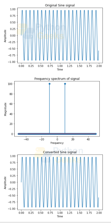
We can see that the original signal and the signal obtained by doing ifft on fft are the same. In this, we are using another function called fftfreq(). This will generate the sampling frequencies.
Special Functions in SciPy
Python provides different functions such as elliptic, convenience functions, gamma, beta, etc., which can be used to do mathematical physics. We can import this sub-package using
from scipy import special
Let us see some of these functions.
1. ERF (erf())
This function is used to calculate the area under a Gaussian curve.
2. Gamma (gamma())
This function calculates the Gamma. The function for this is gamma().
3. Gammaln (gammaln())
This function is used to calculate the log of Gamma.
4. Eppilj (eppilj())
The is used for the elliptic function
5. jn
This represents the Nth order Bessel function. This package also provides exponential and trigonometric functions.
Example of special functions:
from scipy import special

print(special.exp10(5))

print(special.sindg(90))

print(special.cosdg(60))
Output:
1.0
0.49999999999999994
Signal Processing in SciPy
Signal processing involves generating, analyzing, and modifying various signals like sound, image, etc. This subpackage in SciPy can be used to do different operations like designing, filtering, and interpolating one-dimensional and two-dimensional data.
Let us see some of the examples.
Example of resampling:
from scipy import signal
import numpy

t=numpy.linspace(-10,10,20)
sig=numpy.abs(t)
print("Original signal:\n",sig)

print("After resampling:")
print(signal.resample(sig,10))
Output:
[10. 8.94736842 7.89473684 6.84210526 5.78947368 4.73684211
3.68421053 2.63157895 1.57894737 0.52631579 0.52631579 1.57894737
2.63157895 3.68421053 4.73684211 5.78947368 6.84210526 7.89473684
8.94736842 10. ]
After resampling:
[9.97003139 7.84023659 5.8264359 3.67858705 1.51183004 0.5562844
2.6860792 4.69987989 6.84772874 9.01448575]
There are other functions like detrend() to remove the linear element of the signal, order_filter() to perform ordered filtering, etc.
Let us see these examples.
Example of detrending:
from scipy import signal
import numpy

t=numpy.linspace(-10,10,20)
sig=numpy.cos(t)+t
print("Original signal:\n",sig)

print("After detrending:")
print(signal.detrend(sig))
Output:
[-10.83907153 -9.83555659 -7.93548077 -5.99427694 -4.90889369
-4.71239142 -4.54057033 -3.50431676 -1.58709832 0.33834791
1.39097949 1.57079642 1.75884113 2.82785073 4.76129279
6.67005368 7.68993358 7.85399292 8.05918026 9.16092847]
After detrending:
[-0.75029858 -0.79941522 0.04802902 0.93660127 0.96935295 0.11322364
-0.76758685 -0.78396487 0.080622 0.95343665 0.95343665 0.080622
-0.78396487 -0.76758685 0.11322364 0.96935295 0.93660127 0.04802902
-0.79941522 -0.75029858]
Example of ordered filtering:
from scipy import signal
import numpy


sig=np.arange(20).reshape(4, 5)
print("Original signal:\n",sig)

domain = np.identity(3)
print("After filtering:\n")
print(signal.order_filter(sig,domain,1))
Output:
[[ 0 1 2 3 4]
[ 5 6 7 8 9]
[10 11 12 13 14]
[15 16 17 18 19]]
After filtering:
[[ 0. 1. 2. 3. 0.]
[ 5. 6. 7. 8. 3.]
[10. 11. 12. 13. 8.]
[ 0. 10. 11. 12. 13.]]
Image Processing using Python SciPy
SciPy provides a subpackage called ndimage that we can use to perform different operations on the images. These include:
1. Basic manipulations like cropping, flipping, rotating, etc.
2. Image filtering operations like denoising, sharpening, etc.
3. Segmenting image and labeling corresponding pixels
4. Classification of the images
5. Extracting features
6. Registration processes
Now let us see the different functions in this module.
1. Shift – shift(image,(x,y))
This function shifts the image in x and y directions.
2. Rotate – rotate(image, angle)
This function can be used to rotate the image by the specified angle.
3. Zoom- zoom(image, magnitude)
This function can be used to zoom in or out of the image.
4. Median Filter- median_filter(image, argument)
We can use this function to filter an image using a Median filter.
5. Gaussian Filter-gaussian_filter(image, argument)
This function can be used to and a Gaussian filter to the image.
6. Opening an Image in Binary – binary_opening(image)
We can use this function for the binary opening of the image.
7. Closing an Image -binary_closing(opened_image)
We call this function to close the image.
8. Binary Erosion- binary_erosion(image)
We use this function for morphological erosion operation on the image.
9. Binary Dilation- binary_dilation(image)
We use this function for morphological dilation operation on the image
Let us see an example of rotating an image.
Example of image processing:
from scipy import misc,ndimage
import matplotlib.pyplot as plt

img = misc.face() #importing racoon image from the scipy
rotate_img = ndimage.rotate(img, 90) #rotating the image

fig=plt.figure()
plt.imshow(img)
fig=plt.figure()
plt.imshow(rotate_img)
plt.show()
Output:

Optimization
This subpackage contains various optimization algorithms which include:
1. Unconstrained and constrained multivariate, minimization scalar functions like BFGS, Newton Conjugate Gradient, Nelder_mead simplex, etc.
2. Routines for global optimization like differential_evolution, dual_annealing, etc.
3. Least-squares minimization and curve-fitting functions like least_squares, curve_fit, etc.
4. Minimizers of Scalar univariate functions and finders of root(s) like minimize_scalar and root_scalar
5. Algorithms to solve multivariate equation systems like hybrid Powell, Levenberg-Marquardt.
Let us see an example.
Example of optimization:
from scipy.optimize import least_squares
import numpy as np

def func(x):
    return numpy.array([10 * (x[1] - x[0]**2), (1 - x[0])])
arr=np.array([5,5])
result=least_squares(func, arr)
print(result)
Output:
cost: 2.465190328815662e-30
fun: array([-2.22044605e-15, 0.00000000e+00])
grad: array([ 4.44089213e-14, -2.22044605e-14])
jac: array([[-20.00000015, 10. ],
[ -1. , 0. ]])
message: ‘`gtol` termination condition is satisfied.’
nfev: 4
njev: 4
optimality: 4.4408921315878507e-14
status: 1
success: True
x: array([1., 1.])
Statistics in SciPy
Python provides a module consisting of different statistics functions. This is called stats and we can import it by writing the below code.
from scipy import stats
Let us see some of the functions in this module.
1. Cumulative Distribution
We can calculate the cumulative distribution of the set of values using the cdf() function. For example,
Example of cdf:
from scipy.stats import norm
norm.cdf(numpy.array([1,-1.,3,1,0,4,-6,2]))
Output:
5.00000000e-01, 9.99968329e-01, 9.86587645e-10, 9.77249868e-01])
2. Percentage Point
We can calculate the percentage point function of a value using the ppf() function.
Example of ppf:
from scipy.stats import norm
norm.ppf(0.6)
Output:
3. Random Variant Sequence
We can use rvs() function for random variant sequences. For example,
Example of rvs:
from scipy.stats import norm
norm.rvs(size=5)
Output:
4. Binomial Distribution
We can calculate the binomial distribution of the values using the cdf() function.
Example of cdf:
from scipy.stats import uniform
uniform.cdf([1,3,5,7,9],scale=3)
Output:
Interview Questions on Python SciPy
Q1. Write a program to find the solution of the set of linear equations in three variables.
Ans. Below is the example of finding solution of linear equations:
import numpy as np
from scipy import linalg


a = np.array([[2, 1,3], [4,-5,9],[2,-7,4]])

b = np.array([[5], [7],[3]])


x = linalg.solve(a, b)

# Printing the results
for i in x:
    print(i[0],end=',')
Output:
Q2. Find the integration of the sine wave from 0 to pi.
Ans. Below is the example of finding integration:
from scipy import integrate
import numpy


t = np.linspace(0, 1, 20, endpoint = True )
func= lambda t: np.sin( np.pi * t)

integ = integrate.quad(func, 0,1)
print(integ[0])
Output:
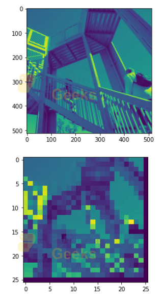
Q3. Write the program to import an image from SciPy and zoom in.
Ans. below is the example of zooming an image :
from scipy import misc,ndimage
import matplotlib.pyplot as plt


img = misc.ascent() #importing  image from the scipy
zoom_img = ndimage.zoom(img, 0.05) #zooming the image by factor 3


fig=plt.figure()
plt.imshow(img)
fig=plt.figure()
plt.imshow(zoom_img)
plt.show()
Output:
Q4. Resample the given signal and show the difference by plotting it.
Ans. below is the example of sampling a signal :
from scipy import signal
import numpy
from matplotlib import pyplot as plt

t=numpy.linspace(-5,5,20)
sig=[]
for i in t:
    sig.append(i**2)

r_sig=signal.resample(sig,30)

fig= plt.figure()
ax1=fig.add_subplot(2,1,1)
ax1.plot(sig)
ax1.set_xlabel('Time')
ax1.set_ylabel('Amplitude')
ax1.title.set_text('Original Signal')
ax2=fig.add_subplot(2,1,2)
ax2.plot(r_sig)
ax2.set_xlabel('Time')
ax2.set_ylabel('Amplitude')
ax2.title.set_text('Resampled Signal')

fig.tight_layout()
plt.show()
Output:

Q5. Find the uniform distribution of a set of values using modules in the SciPy package.
Ans. Below is the example of finding uniform distribution :
from scipy.stats import uniform
print (uniform.cdf([ 1, 5, 3, 9, 125], loc = 1, scale = 4))
Output:
Quiz on Python SciPy
Conclusion
We have learned about the SciPy module, its applications. And also different sub-packages that contain tools to perform different operations. We also saw some practice problems.
Hope you understood the concepts covered in this article. Happy learning!

1. Solving a set of linear equations:
Let us say we want to solve two equations in x,y 2x+y=5 4y-5x=7.
# Creating the input array
a = np.array([[2, 1], [4,-5]]) #SHOULD BE a = np.array([[2, 1], [-5,4]])
Output:
[[2.28571429]
[0.42857143]]
Should be:
[[1.]
[3.]]