Probability Distribution using Python

In this article, we will learn about probability distribution using Python. We will look at the four major probability distributions: normal distributions, normal distributions, poisson distributions and bernoulli distributions. We will also learn how to implement probability distributions in python. So let’s begin.

What do you mean by Probability distribution?

Most statistical tools and techniques we use in data analysis are based on probability. Probability tells us how likely an event is to occur on a scale of 0 to 1. 0 means the event never occurs, and one indicates the event always occurs. Variables in the probability vary based on chance.

The probability distribution tells us how distributed a random variable is. As a result, we can understand what values it will most likely take and what values it is likely to take.

What is a Random variable?

A random variable is a quantity produced by a random process. In probability, a random variable takes many possible values—for example, events from a state space. We denote the random variables using a capital letter. Values the random variable takes are denoted using lowercase letters along with an index.

There are three major types of random variables:

1. Discrete RV: the values are taken from a finite set of states.

2. Boolean: the values are either true or false.

3. Continuous: the values are taken from an infinite set of states

Implementing probability distribution using Python

Let us look at how to implement probability distributions using python:

1. Normal probability distribution

The normal distribution is also called the Gaussian distribution. It gives a bell-shaped curve in statistical reports and is one of the required probability distributions. It is a continuous probability distribution that is symmetrical around its mean. The values away from the mean on both sides narrow the curve.

Examples of the normal distribution are height, weight, blood pressure, IQ scores and so on.

We use the python numpy library to implement the distribution.

random.normal() method– we use this method to get the normal data distribution.

It has three parameters:

• Loc– this is the mean and the point where the bell exists.
• Scale– this is the standard deviation. It tells how flat the graph should be.
• Size– gives the shape of the returned array.

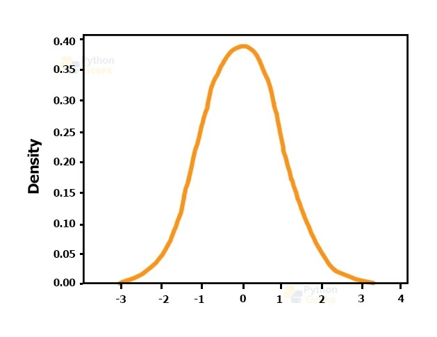
Visualisation of normal distribution using Python

The following code gives an idea about how to work with normal distributions:

From numpy import random
Import matplotlib.pyplot as plt
Import seaborn as sns
sns.distplot(random.normal(size=1000),hist=False)
plt.show()

Output

2. Binomial distribution

We use the binomial distribution when we have exactly two mutually exclusive outcomes of a trial. We label these outcomes as “success” and “failure”. The binomial distribution obtains the probability of observing x successes in N trials. A single trial’s probability of success is denoted by p. The distribution has a fixed p for all trials.

This is a discrete distribution. It gives the outcomes for binary cases. For example, tossing a coin gives the outcome as heads or tails.

It has three parameters:

• n – total number of trials.
• p – the probability of occurrence of each trial.
• Size – the shape of the returned array.

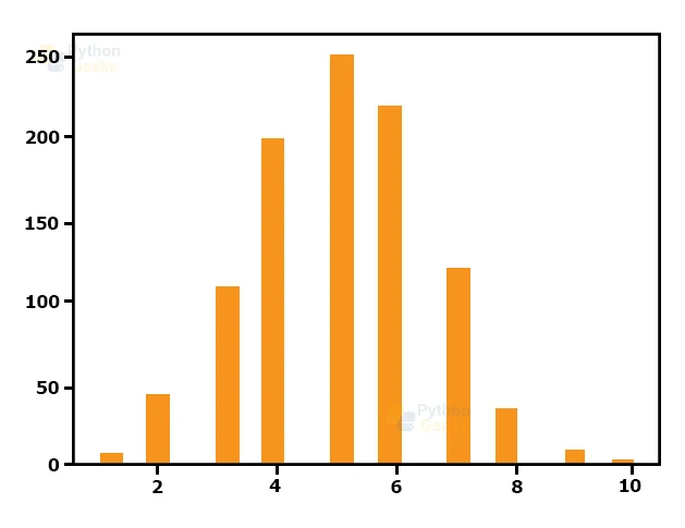
Visualisation of the binomial distribution using Python

From numpy import random
Import matplotlib.pyplot as plt
Import seaborn as sns
sns.distplot(random.binomial(n=10, p=0.5, size=1000), hist= True, kde= False)
plt.show()

Output

3. Poisson distribution

When we know how often the event has occurred, the poisson distribution helps predict the probability of a certain event. Poisson distribution tells us the probability of a given number of events occurring in a fixed time interval.

Examples of Poisson distribution include predicting the probability that more books will sell, predicting the weather forecasts, estimating flight and hotel prices and so on.

The distribution has two parameters:

• Lam– the number of known occurrences.
• Size– the shape of the returned array.

Visualisation of the poisson distribution using Python

From numpy import random
Import matplotlib.pyplot as plt
Import seaborn as sns
sns.distplot(random.poisson(lam=2,size=1000), kde=False)
plt.show()

Output

4. Bernoulli distribution

Bernoulli distribution is a unique case of Binomial distribution. The number of distributions is 1 for a single experiment which is conducted. Bernoulli distribution is for events with two outcomes.

The numpy library consists of various functions to plot a Bernoulli distribution. The probability distribution curve is created over the histogram.

Visualisation of the bernoulli distribution using Python

From scipy.stats import bernoulli
Import seaborn as sb
data_bern=bernoulli.rvs(size=1000, p=0.6)
ax=sb.distplot(data_bern, kde=True, color=green, hist_kws={‘linewidth’:25,’alpha’:1})
ax.set(xlabel=’bernoulli’,ylable=’frequency’)

Output

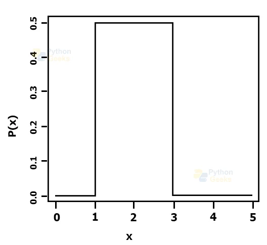
5. Uniform distribution

Uniform distribution is a simple yet highly useful distribution. The probability distribution function is as follows:

f(x) = 1/(b-a)            for a<=x<=b

and

f(x) = 0                       for x<a or x>b

It has a constant probability, and it is also called the rectangular distribution function.

The function is defined by two parameters:

• A is the minimum.
• B is the maximum.

Uniform distribution in python

A random number generator acts over the intervals of a and b. This helps users to visualize the python distribution.

You need to import the following code from the scipy.stats module. We get the distribution using the log and scale parameters.

6. Gamma distribution

The gamma distribution is a continuous distribution that can model many different things. We start by importing numpy as np as it contains the gamma distribution. The parameters are the shape, scale and size.

7. Exponential distribution

We begin by importing the two libraries numpy and matplotlib. Then we define a variable to store the arrange function. This function will make a series of values that starts and ends at the specified values. Then we multiply all the exponential values by four and give them to the amplifier variable we create. Then we plot the distribution.

Types of data

We work with many types of data formats in machine learning. The datasets we use in machine learning contain different kinds of textual, imagery and video data from billions and billions of different sources.

We must identify patterns to make predictions for the entire dataset or populations.

Generally, the data is classified into the following ways:

1. Numerical: this includes integers, floating point numbers and so on. It is further classified into the following types: discrete and continuous.

2. Categorical: this type of data contains labels such as names, genders, etc. It can be binary or multi-valued.

Elements of the probability distribution

We use the following probability functions to get probability distributions:

Probability mass function: the solution of the mass function lies in values that are discrete random variables. It is also known as a discrete probability distribution.

Probability distribution function: the solution of the mass function lies in values that are continuous random variables. It is also known as a continuous probability distribution.

Conclusion

In this article, we saw what probability distributions are, the different kinds of probability distributions and finally, how to implement the distributions using python. We hope our explanation was easy to understand.