Popular Search Algorithms in AI

Artificial Intelligence is the science of creating rational agents. To do their responsibilities, these agents almost always use a search algorithm in the background.

With the help of these agents, problems of great combinatorial complexity can be solved. Because a problem can have multiple solutions, these agents search space for all possible combinations and employ techniques to identify the shortest path or the most appropriate path to the end goal.

As a result, Search, in conjunction with agents, plays a critical role in Artificial Intelligence. Search guarantees that the AI machine/system functions correctly by providing a conceptual backbone for various searching strategies and algorithms, as well as performing a methodical investigation of possibilities.

But!

What is the nature of the search algorithm? What are the different sorts of search algorithms? Why are they so important when it comes to problem-solving?

These and other questions will be addressed in the following debate on Search Algorithms. But, before we get into search algorithms, let’s take a closer look at AI search and how it works.

What is Search in Artificial Intelligence?

Search, whether in AI or in general, is a step-by-step method for resolving a search problem in a specific search space. It accomplishes this by examining several aspects of the search problem, including:

1. Search Space

In the initial state of the search issue, the search space represents all of the conceivable sets of solutions that a system could have.

2. Start State

This is where the agents start their search.

3. Target Test

This is the final state of the search problem; it observes the current state of the problem space and returns whether or not the goal state has been reached.

Following the completion of these factors, the solution to the search issues is offered in the form of a plan, which transforms the start state to the target state. The role of search algorithms begins here since it aids in the execution of the plan.

What is Search Algorithm?

Whether it was ‘Deep Blue’ eliminating Gary Kasparov in chess in 1997 or ‘Alpha Go’ defeating Lee Sudol in 2016, AI’s ability to mimic and surpass human mental powers has grown tremendously.

Such Artificial Intelligence programs are built around search algorithms. While we may be tempted to believe that this is solely useful in the realms of gaming and puzzle-solving, such algorithms are employed in a wide range of AI applications, including action planning, robotics, software, autonomous driving, theorem proving, and so on.

Many AI problems can be modeled as a search problem, with the aim being to get from the original state to the destination via state transformation rules.

So, in a nutshell, the search space is a graph (or a tree), and the purpose is to get from the beginning state to the end by taking the shortest path, in terms of cost, length, etc.

AI Search Algorithm Terminologies

1. Problem Space

It is, in essence, the setting in which the search takes place. (A set of states and a set of operators for changing them.)

2. The instance of the Problem

It’s a result of the initial state plus the target state.

3. Graph of Problem Space

We utilize it to indicate the status of a situation. We also use hubs to represent states, whereas edges represent operators.

4. The gravity of a problem

The length of the shortest possible path can be determined.

5. Complexity of Space

We can calculate it as the greatest number of hubs stored in memory.

6. Complexity of Time

The greatest extreme number of hubs produced is defined.

7. Applicability

It can be described as a quality of a calculation that allows it to consistently find an optimum layout.

8. Factor of Stretching

In the problematic space diagram, we can determine it as the typical number of youngster hubs.

9. Depth

The distance between an underlying state and an objective state can be traveled in the least amount of time.

Brute-Force Searching Tactics

This method does not necessitate domain-specific expertise. As a result, it’s a straightforward method. As a result, it runs smoothly and reliably with a limited number of possible states.

Brute Force Algorithm Requirements

• A description of the state
• A list of valid operators
• Beginning State
• Goal state description

Properties of Search Algorithms

The following are the four essential qualities of search algorithms that can be used to compare the effectiveness of various algorithms:

1. Completeness

If a search method guarantees to return a solution if at least one solution exists for any random input, it is said to be complete.

2. Optimality

A solution obtained for an algorithm is considered to be optimal if it is guaranteed to be the best solution (lowest route cost) among all other solutions.

3. Time Complexity

It is a measure of how long it takes an algorithm to perform its task.

4. Space Complexity

The maximum storage capacity required at any time during the search, as measured by the problem’s complexity.

Types Of Search Algorithms In AI

There are many different types of search algorithms in Artificial Intelligence. However, they are divided into two groups, each of which differs significantly from the other. While some use a priority queue or a root note, others use a closed list or an open list of nodes.

These types of search algorithms are:

1. Uniformed Search

Uniformed Search, also known as Blind Search or Brute-Force Search, has no domain expertise that can assist it in achieving the goal other than that which is provided in the problem statement.

This sort of search algorithm is just concerned with attaining the objective and achieving success, and it may be applied to a wide range of search algorithms because the target problem is unimportant.

This way of searching is further subdivided into the following categories:

• Breadth-First Search
• Uniform Cost Search
• Depth First Search
• Iterative Deepening Search
• Bidirectional Search

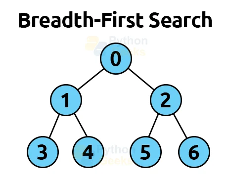
a. Breadth-First Search

This is an AI search technique that traverses a tree in a breadthwise manner to find the goal.

This calculation selects a single hub (beginning or source point) in a chart and then visits all of the hubs that are nearby.

When the calculation identifies the starting hub, it then proceeds to the nearest unvisited hubs and examines them. All hubs are stamped once they’ve been visited.

These emphases continue until all of the chart’s hubs have been visited and checked thoroughly. Because a FIFO(First In First Out) queue data structure can be used to implement this search. The quickest path to the solution is provided by this method.

Disadvantages of Breadth-First Search

• Because each level of the tree must be saved into memory before moving on to the next, it necessitates a large amount of memory.
• When the solution is located distant from the root node, BFS takes a long time.

b. Depth-First Search

It is a search algorithm that traverses the search tree from the root node. The Last In First Out (LIFO) principle is used.

As a result, it produced the same number of nodes as the Breadth-First technique, but in a different order.

It will be traversing, looking for a key at a specific branch’s leaf. If the key is not located, the search goes back to the place where the other branch was left unexplored, and the process is repeated for that branch as well.

Disadvantages of DFS

• Many states are likely to repeat, and there is no guarantee that a solution will be found.
• Deep searching is performed via the DFS algorithm, which can occasionally enter an infinite loop.
• In any instance, if d is smaller than the defined cut-off, the execution time will increase.
• Its multidimensional nature is based on a variety of factors. It is unable to check copy hubs.

c. Uniform Cost Search Iterative

When the step costs are not the same yet we need the best solution to the objective state, this algorithm is utilized. It also grows the lowest-cost hub on a continual basis. It does not search for the next node with the lowest cost; instead, it searches for the next node with the lowest cost.

Disadvantages of Uniform Cost Search Iterative

• It is just concerned with the path cost and is unconcerned with the number of steps required in the search. As a result, this algorithm may become trapped in a never-ending loop.

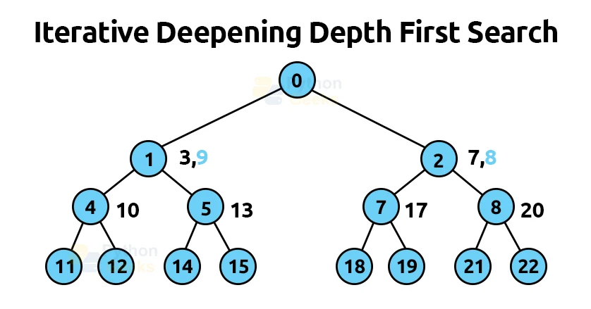
d. Iterative Deepening Depth First Search

It’s a search algorithm that combines the BFS and DFS algorithms’ strengths. It is an iterative process. In each iteration, it looks for the best depth. It follows the Algorithm till it reaches the destination node. The algorithm is programmed to search until it reaches a particular depth, which increases with each iteration until it achieves the desired state.

Disadvantages of Iterative Deepening DFS

• The biggest disadvantage of IDDFS is that it duplicates all of the preceding phase’s work.

e. Bidirectional Search Algorithm

As the name implies, Bidirectional Search is a combination of forwarding and backward search.

Both searches should put the information structure in jeopardy. It uses a guided chart to find the shortest route from the source (initial hub) to the destination hub.

The two missions will start from separate locations, and the calculation will come to a halt when the two inquiries intersect at a hub. It is a faster technique that reduces the amount of time spent navigating the diagram.

Disadvantages of bidirectional search algorithm

• The implementation of the bidirectional search tree is complex.
• In bidirectional search, the objective state should be known ahead of time.

Comparison of the Complexities of Different AI Search Algorithms

Let’s have a look at how algorithms are performed based on various criteria.

Criterion	Breadth-First	Depth First	Bidirectional	Uniform Cost	Interactive Deepening
Time	bd	bm	bd/2	bd	bd
Space	bd	bm	bd/2	bd	bd
Optimality	Yes	No	Yes	Yes	Yes
Completeness	Yes	No	Yes	Yes	Yes

2. Informed Search or Heuristic Search

Also known as Heuristic Search, this sort of search algorithm makes use of domain knowledge and employs a heuristic function to calculate the cost of the optimal path between two states as well as the proximity of each state to the goal.

Informed search can be separated into two types:

• A* Search
• Greedy Search

Functions of Heuristic Evaluation

They work out the cost of the quickest path between the two states. For sliding-tiles games, a heuristic function is calculated by calculating the number of moves each tile makes from its goal state and adding these numbers for all tiles.

Pure Heuristic Search

It grows nodes in the order in which their heuristic values appear on the graph. It generates two lists: a closed list for nodes that have already been expanded and an open list for nodes that have been generated but have not yet been enlarged.

Each iteration expands a node with the lowest heuristic value, creates all of its child nodes, and places them in the closed list. The heuristic function is then applied to the child nodes, and their heuristic value is used to determine where they belong in the open list. Shorter pathways are saved, while longer paths are discarded.

a. A* Search Algorithm

The most well-known type of best-first pursuit is the A* search. It makes use of heuristic capacity h(n) and the cost of getting to the hub n from the starting state g. (n). It combines the advantages of UCS and avaricious best-first inquiry to effectively address the problem.

Using the heuristic capacity, an A* search calculation finds the shortest path through the hunt space. This hunt computation uses fewer chase trees and produces a perfect result faster.

f(n) = g(n) + h(n)

where g(n) is the cost of getting to the node,
h(n) is the expected cost of getting from the node to the goal,
f(n) is the estimated total cost of the path from n to goal.

A* computation is similar to UCS except it uses g(n)+h(n) instead of g. (n) description.

b. Greedy Best First Search Algorithm

The nearest node to the goal node is extended in greedy search methods. A heuristic function h is used to compute the proximity factor (n). The distance between one node and the end or goal node is estimated by h(n). The closer the node is to the endpoint, the smaller the value of h(n). When the greedy search is looking for the best path to the goal node, nodes with the lowest possible values are chosen. However, f(n) = h(n) is required for node explanation.

3. Local Search Algorithm

In Artificial Intelligence, local search is an optimization algorithm that finds the best solution more quickly. When we just worry about the solution and not the journey to it, we employ local search methods. Local search is utilized in the majority of AI models to find the best answer based on the model’s cost function. In linear regression, neural networks, and clustering models, local search is applied.

4. Hill-Climbing Searching

It is an iterative algorithm that begins with an arbitrary solution to a problem and strives to improve it by slowly modifying one aspect of the answer. An incremental adjustment is considered a new solution if it results in a superior solution. This method is continued until no additional improvements can be made.

Hill-Climbing (problem) is a function that returns a state that is a local maximum.

5. Local Beam Search

This algorithm maintains a total of k states at any given time. These states are generated at random at first. The goal function is used to calculate the successors of these k states. The process comes to a halt if any of these successors is the maximum value of the objective function.

Otherwise, the states are arranged in a pool (initial k states and k number of successors of the states = 2k). The pool is then numerically sorted. As new beginning states, the highest k states are chosen. This method is repeated until the maximum value has been reached.

A solution state is returned by the function BeamSearch(problem, k).

6. Simulated Annealing

Annealing is a process that involves heating and cooling metal to modify its interior structure and alter its physical properties.
When the metal cools, its new structure is preserved, and the metal retains its newly acquired qualities. The temperature is not fixed in the Simulated Annealing Process.

We start with a high temperature and then let it gradually ‘cool’ as the calculation progresses. When the temperature is high, the computation allows for optimally smaller solutions.

Start

Set k = 0; L = integer number of variables;
From i → j, find the performance difference.
If Δ <= 0 then accept else if exp(-Δ/T(k)) > random(0,1) then accept;
For L(k) steps, repeat steps 1 and 2.
k = k + 1;
Steps 1 through 4 must be repeated until the criteria are met.

End

The Traveling Salesman Problem

The basic question in the traveling salesman problem is: “When cities with distances between them are specified, the main purpose is to discover the shortest route from City A to City B.” For a visual reference, see the diagram.

Start
Find all (n – 1) possible configurations, where n is the total number of urban communities. Also, get the basic cost by calculating the cost of each of these (n – 1)! configurations. Finally, keep the one that has spent the least amount of money.
End

Conclusion

In essence, we have considered Popular Search Algorithms in AI. The repetitive, manual chores that do not demand a lot of capacity but can be reasonably simply optimized are the ones that are likely to be affected by the transition.

We hope that this page has covered the majority, if not all, of the prominent AI search algorithms.