Neural Network Learning Rules
Get Ready for Your Dream Job: Click, Learn, Succeed, Start Now!
As seen earlier, the ANN model is greatly inspired by the way a biological neural network works. It tends to imitate the way in which the human is capable of making logical decisions and adaptations. We’ve seen till now that ANNs tend to form a model that has a similar structure to the human brain.
Similar to the biological neural network, Artificial Neural Network has the counterparts like nodes, input, and output for the corresponding functions of senses, processing, and decision making. However, only having the same structure as a biological neural network doesn’t help ANNs in making human-like logical decisions. In order to do so, the Neural Network has to function like a real Brain.
Scientific studies prove that the greatest virtue of the Brain is its ability to retain things and “learn ” new things. The process of “learning” is nothing but adapting to new environments and retaining the results for further usage. Consequently, if we want the ANNs to behave like the way in which the brain works, then we have to use these algorithms to “learn” new things. In order to do so, a set of “learning rules” are devised to help the algorithms to learn.
In this article, PythonGeeks brings to you a detailed introduction to the learning rules in Neural Networks. We will learn what are learning rules, various learning rules, and their mathematical connection between the weights and the biases. Therefore, let’s dive into the article and learn more about the rules.
Introduction to Neural Network Learning Rules
ANNs tend to acquire characteristics similar to that of a biological network. In its primitive or base form, the Brain tends to modify its neural structure in order to learn. It manages to alter the competence of its synaptic connections depending on the activities it has to perform. In order to help ANN replicate this behavior, we need to alter the neural structure of this Network as well. With this intention in mind, the main idea behind changing the neural structure of the network is to alter the input and output variables of the network.
As we have seen earlier, ANN inputs and outputs are a function of their weights and biases. Since we fix the weights and biases prior to the execution, it becomes difficult for us to try and alter the input and output. In an attempt to achieve so, we try applying various mathematical logics and methods to alter the weights associated with the different layers of the network. These rules are “Learning Rules”. Thus, in simple words, Learning Rules are mathematical rules that change the weights and biases of the levels when a network simulates in a specific data environment. This is an iterative process. It helps the neural network to “learn” from the prevailing conditions which in turn improves its performance.
Now that we know what these Learning Rules are, let us look at the different Learning Rules in detail.
Gradient Descent Learning
In this type of learning, the error reduction takes place with the help of weights and the activation function of the network that we want to develop. The only criteria that the function has to follow is that the activation function should be differentiable.
We perform the adjustments of weights depending on the error gradient E that we observe in this learning. The backpropagation rule is one of the many examples of this type of learning. Thus the weight adjustment is:
ΔW = 𝝰(𝛿E/𝛿W) where 𝞪 is the learning rate and (𝛿E/𝛿W) is the error gradient with respect to W.
Stochastic Learning
In this type of learning, we have to deal with two types of unsupervised learning. They are the Hebbian Learning Rule and the Competitive Learning Rule.
Hebbian Learning Rule
Developed in 1949 by Donald Hebb, Hebbian Learning Rule was the primary learning rule then. It is an unsupervised neural network learning algorithm. The primary motive of this algorithm is to determine the relationship between the improvement and the weights of the nodes of the network.
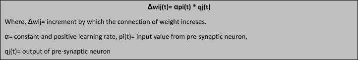
The rule assumes that if two neighboring nodes activate or deactivate at the same time, then the weight that connects them increases. Similarly, for neutrons operating in opposite phases, i.e., if one of them activates and the other one deactivates at the same time, then the weights connecting them decreases. Apart from this, if the neutrons do not have a signal connection between them, then there should be no change in the weight.
To elaborate, if inputs of the two nodes are either positive or negative at the same time, then a strong positive weight should subsist between them. Similarly, if the nodes are in opposite phases, i.e., if one of them is positive while the other one is negative then, a strong negative weight should subsist between them.
In the beginning, all the weights are set to a zero value. It is an ideal algorithm for both hard as well as easy activation functions. Since we do not utilize the desired actions of the neutrons in the learning process, we categorize this under unsupervised learning rules. The absolute values of the weights are directly linked with their learning time.
Single Neuron Perceptron: As our brain is capable of handling larger and variant information at any given point, computer models can also tend to solve problems with a structural variation of the algorithms like classification, regression, and others. Inspired by this behavior, ANNs tend to imitate the structure of a single processing unit of the brain (neuron). This single neuron model is capable of handling larger units of input data. Single neuron perceptron classified its input into two classes, null and 1.
Multiple Neuron Perceptron: Perceptron models with multiple neurons handle the query in a different way as compared to the single neuron model. Each neuron of the multiple neuron perceptron has a decision boundary associated with it. These boundaries help in making better logical decisions. Unlike single neuron perceptron, multiple neuron perceptron is capable of classifying its data into more than two classes.
According to the Hebbian Rule, the mathematical deviation of the rule is as follows:
Perceptron Learning Rule
With the variation in the applications of the supervised learning algorithm like classification, regression, pattern recognition, and others, the approach in which they can be executed can also be varying. It includes variations of all kinds like structural, statistical, and neural approaches. Along with these, ANNs are stirred by the physiology of the human brain as well. They not only try to imitate the working of the whole brain but also try to replicate the scientific model of a single neuron and thus try to reproduce the working of the Brain.
This rule is a mistake correction algorithm for the supervised learning algorithm of the single-layer feedforward networks with a linear activation function. As the nature of the algorithm is supervised, the algorithm compares the variation between the actual and the expected output in an attempt to calculate the error. If in any case, we encounter an error, then it is inferred that an alteration is required in the weights of the connections.
Mathematical interpretation: To understand the algorithm in its mathematical form, let us consider the below case. Consider that we have ‘n’ arbitrary finite inputs. Let xn be the input vector and tn be the target-based time, then the output ‘y’ can be given as:
y= f(yin)= 1 for yin>θ or 0 for yin<θ where θ is the threshold value
We update the weight as
w(new)= w(old)= tx {where t≠y}
No change in weight {where t=y}
Delta Learning Rule
Also known as the Least Mean Square or LMS rule, Delta Rule was given by Bernard Widrow and Marcian Hoff. It minimizes the error expanding over the entire training pattern. It has a continuous activation function and is an example of a Supervised Learning algorithm.
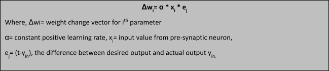
The base of the rule lies in the gradient-descent approach. The algorithm tends to compare the input vectors and the variations in the output vector. If the difference between the expected and actual output vector is not significant or not there, then the weights between the connections are unaffected. Whereas, if we observe any difference then we have to alter the weights in such a way that the difference is null or insignificant.
In other words, if we do not observe any difference in the output vectors, then the learning will not take place. It is also seen that when we plot the graph of the weight of a network with linear activation function and no hidden input against the squared difference, then we get a paraboloid in the n-space. As the proportionality constant is also negative, the graph that we achieve is a concave upward graph and thus it has the least value associated with it. The vertex of this graph is the area where we achieve the region of lowest possible error. The weight vector that corresponds to such a vertex point is the ideal weight that we need to consider.
The mathematical representation of the rule goes as:
Correlation Learning Rule
The Correlation Learning Rule is loosely based on the same principle as that of the Hebbian Learning Rule. Similar to the Hebbian Rule, it assumes that if the connection between the neurons is similar then the weights between them should increase, whereas, if they show a negative relationship, then the weight between them should decrease.
The rule differs from the Hebbian Rule on one basis. The Hebbian Rule is an unsupervised learning rule while Correlation Rule is a Supervised Learning Rule. The mathematical representation of the rule is given by:

Competitive Learning Rule
We can classify the Competitive Learning Rule under Unsupervised Learning. In this type of learning model, the nodes at each tend to dominate the formation of the input pattern. The basis of this rule is “Winner takes it all”. Here, the input with the highest activation function will have dominance in the formation of the output pattern. We know this rule as “winner takes it all” because of one more reason, only those neurons which are responsible for the output formation change at end of the cycle. The neurons which did not participate in the output remain unaffected.
The mathematical formulation of this rule for selection of the winner neuron, condition for sum total weight, and the formula for the affected neurons are:
- Condition to decide the winner: yk = 1 if vk> vj or yk= 0 in all other cases.
Here, if the neuron yk wants to be the winner then its induced local field (vk) should be greater than the induced local field of other neurons(vj). - Condition for Sum total of weights: Another constraint for the neuron k in this learning rule is that
Σ wkj= 1 for all k. - Change of weight: The change that occurs in the weights that are a part of the output pattern formation is
Δwkj=- 𝞪(xj – wkj) if neuron k is the winner or 0 if it does not win.
Out Star Learning Rule
Out Star Learning Rule is a supervised learning rule given by Grossberg. We use this algorithm when we adopt that the neurons present in a network are arranged in a consecutive layer. In this learning rule, the weight associated with a particular node should be equal to the desired output for neurons that are connected to the weight.
The mathematical representation of the rule is:

Conclusion
To conclude this article, we can certainly say that learning rules in ANNs are certainly a crucial step in helping machines to learn. We came to know how the Brain alters its neural structure to adapt to the learning algorithm. In a similar attempt, we use learning rules to help Machines change their weights which in turn changes its output. This helps Machines in adapting to the Learning Environment. Hence, we came across the various rules that are available for the purpose.
