Machine Learning Project – Breast Cancer Classification

What is Breast Cancer?

Breast cancer is a prevalent form of cancer that affects both men and women, although it is very rare in men compared to women. Machine learning techniques are employed to analyse vast patient datasets to aid medical professionals in producing accurate diagnoses and customising treatment plans.

Breast cancer classification is achieved through the implementation of machine learning techniques like decision trees, neural networks and support vector machines. These techniques use supervised learning methods on a large dataset to identify deep patterns and relationships that are not easily identifiable by human experts.

Alternatively, the use of unsupervised algorithms for clustering purposes can be employed alongside dimensionality reduction techniques. By training on massive datasets, these algorithms are capable of detecting connections and patterns, which would eventually help in the process of breast cancer classification.

Dataset

The Breast Cancer Classification dataset is a collection of data containing breast cancer cases, including benign and malignant tumours. The dataset includes characteristics such as the radius of lobes, the outer perimeter of lobes, etc. The information was gathered from several clinical sources and put into a single dataset for research purposes. The dataset may be used to train machine learning algorithms to identify breast tumours as benign or malignant based on the numerous characteristics supplied.

This dataset is useful for academics and students working on breast cancer detection and classification. It may be utilised to create new machine-learning algorithms and models for the early identification of breast cancer.

The dataset can be downloaded here. Link

Prerequisites for Breast Cancer Classification Using ML

The project makes use of the following Python libraries:

• NumPy
• Pandas
• Matplotlib
• Seaborn
• Scikit-Learn

Download Machine Learning Breast Cancer Classification Project

Please download the source code of Machine Learning Breast Cancer Classification Project: Machine Learning Breast Cancer Classification Project Code

Steps for Machine Learning Breast Cancer Classification Project

1. Importing the required libraries.

import numpy as np 
import pandas as pd 
import seaborn as sns
import matplotlib.pyplot as plt
sns.set_theme(style="whitegrid")

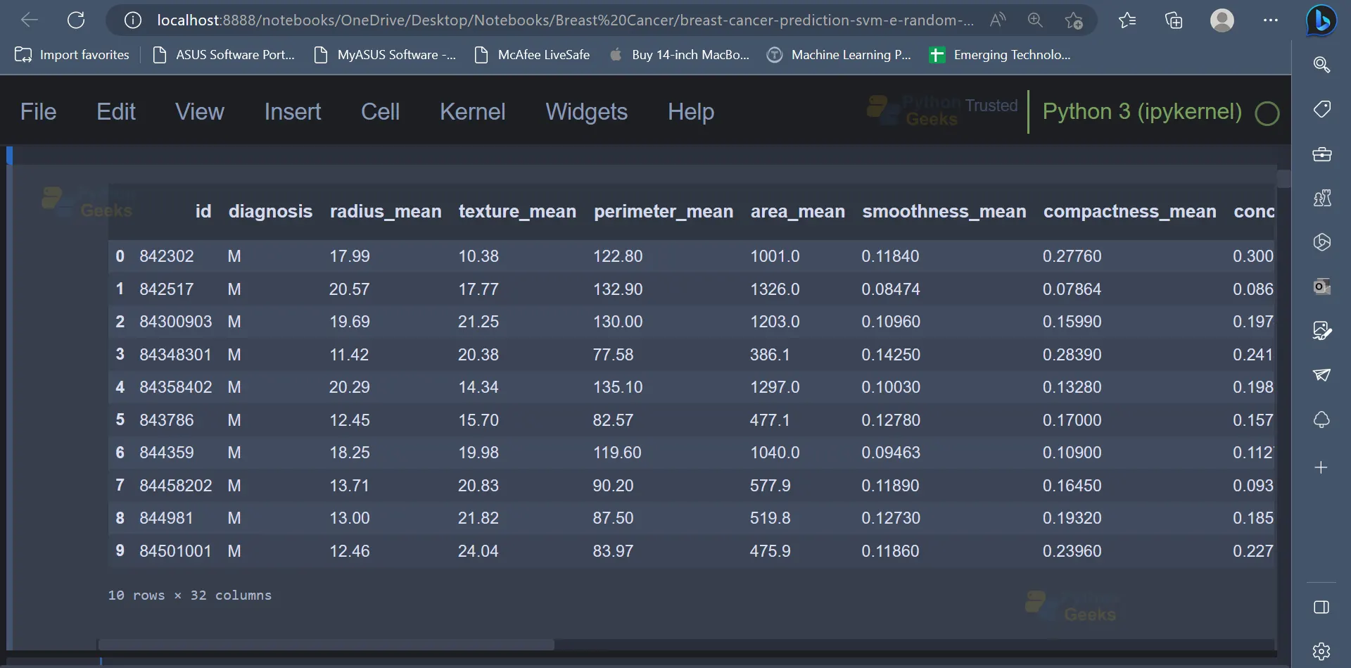
2. Once the necessary libraries have been imported, the next step would be to read the dataset and display the dataset as well. The first ten rows have been displayed in the screenshot shown below. The dataset contains features like radius_mean (radius of the lobes), perimeter_mean(outer perimeter of lobes), diagnosis( indicates whether a person has a malignant tumour or benign tumour), etc.

# Reading the Dataset
data = pd.read_csv('breast-cancer.csv')
data.head(10)

Output

3. Sometimes, the dataset may contain unnecessary columns, which will have to be removed from the dataset before we use the dataset to train Machine Learning models.

# Removing columns that will not be used
data = data[[c for c in data.columns if (('_se' not in c) and ('_worst' not in c))]]
data.drop('id', axis=1, inplace=True)

4. Let’s go ahead and explore the dataset by carrying out some Exploratory Data Analysis.

data.info()

Output

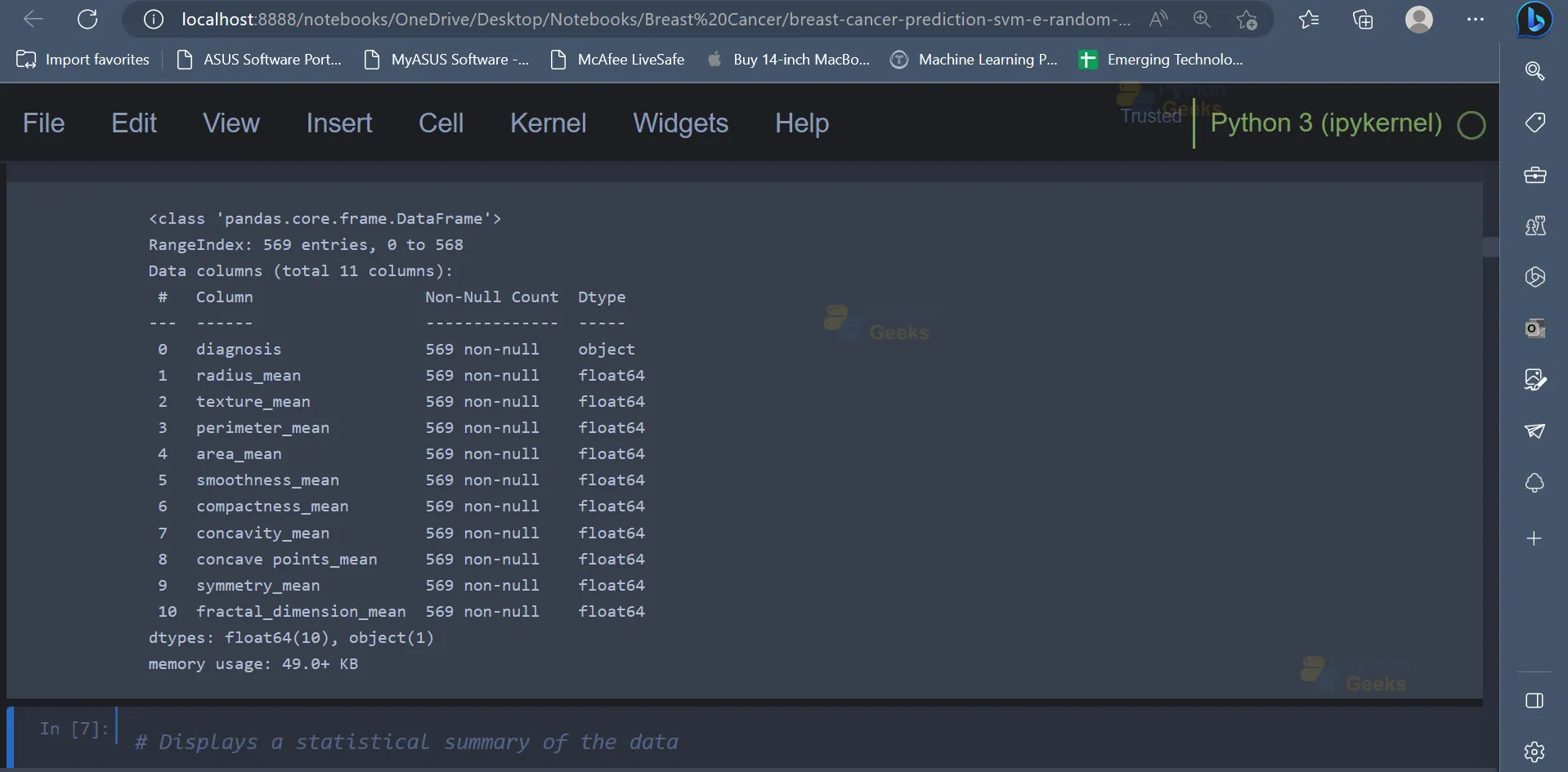
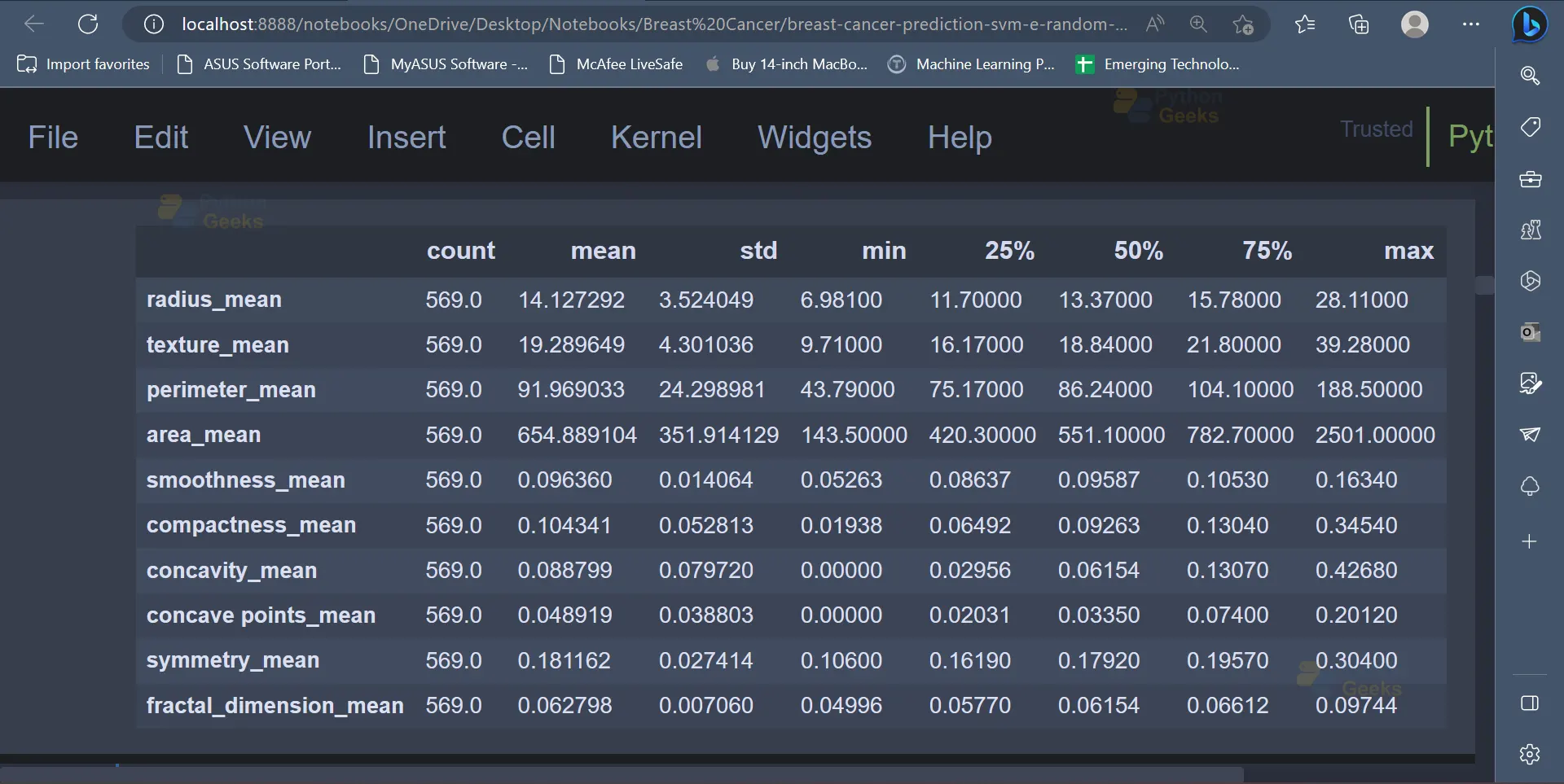
5. The dataset contains 569 entries, and there are 11 attributes/columns present in the dataset. The describe() function can be used to get a statistical summary of the data.

# Displays a statistical summary of the data
data.describe().transpose()

Output

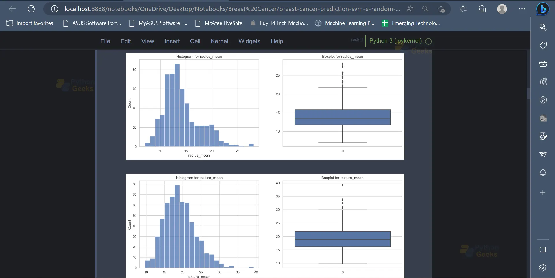
6. Now that we have some statistical insights about the data, it’s time to represent this data in a visually appealing format with the help of some graphs and charts. Histograms and boxplots are two amazing ways to represent data in the form of a graph. A custom function can be declared to plot the histogram as well as a boxplot for the values of a given attribute/column present in the dataset.

# Defining the function to display the boxplot and histogram graphs
def hist_box_plot(df, column, height=15, width=5):
    fig, axes = plt.subplots(1, 2, figsize=(height, width))
    sns.histplot(ax=axes[0], data = df
);
    axes[0].set_title(f'Histogram for {column}')
    sns.boxplot(ax=axes[1], data = df
);
    axes[1].set_title(f'Boxplot for {column}')
    plt.show();

This function can then be applied for all the columns present in the dataset except the diagnosis column since the diagnosis column contains only string values which indicate the two classes of breast cancer (Malignant or Benign).

for col in data.columns[1:]:
    hist_box_plot(data, column=col)

Output

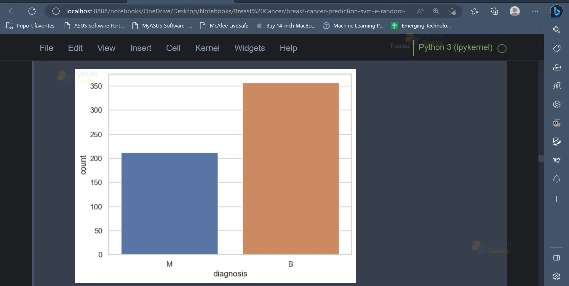
7. As mentioned earlier, the diagnosis column is the target column, and it contains two values, M and B, which indicate whether the tumour is malignant or benign in nature. We can have a look at the ratio of the number of rows having a value of M in the diagnosis column to the number of rows having a value of B in the diagnosis column.

sns.countplot(data=data, x='diagnosis');

Output

8. In the next step, we will create a copy of the data. This is done in order to have a backup of the original data in case some data is lost accidentally. Once this is done, the string values in the diagnosis column (‘M’, ‘B’) can be converted into integer values (1, 0) so that they can be easily understood by machine learning models.

data_copy = data.copy()
data_copy['diagnosis'] = data_copy['diagnosis'].map({'M': 1, 'B': 0})

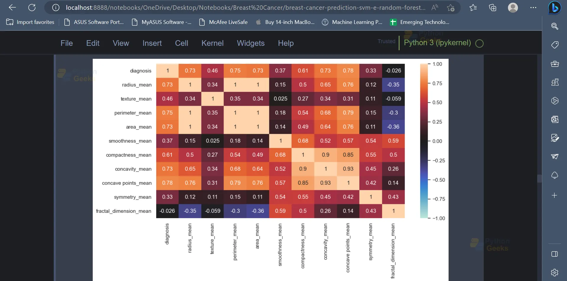
9. The correlation matrix indicates the relationship between various variables present in the dataset and how each variable is affected by every other variable. It can also be plotted using the below code.

# Displays a heat map based on the correlation coefficient of the variables
corr = data_copy.corr('spearman')
plt.figure(figsize=(12, 6))
sns.heatmap(corr, vmin=-1, center=0, vmax=1, annot=True);

Output

10. Feature engineering is an important step in any machine learning project. In this step, the important features from the dataset will be selected. These features will then be used to train various machine-learning models.

# Independent variables (predictors)
X = data_copy.drop('diagnosis', axis=1)
# Dependent variable
y = data_copy['diagnosis']

11. The dataset contains attributes which belong to a wide range. It would be convenient to have all the values belonging to a similar range or a similar scale, which would eventually help the machine learning model understand the data in a better way. The MinMaxScaler can be used for this purpose, as shown below.

from sklearn.preprocessing import StandardScaler, MinMaxScaler
# Data Standardization
scaler = MinMaxScaler()
X = scaler.fit_transform(X)

12. Now, the data can be split into training data and testing data. The training data can be used to train various machine learning models, and the testing data can be used to analyse the performance of the models.

# Train Test Split
X_train, X_test, y_train, y_test = train_test_split(X, y, test_size=0.2, random_state=123)

13. Once the data is split into training data and testing data, various machine learning models can be trained using the training data. We will be using models like Logistic Regression, Decision Tree, SVM, etc.

from sklearn.linear_model import LogisticRegression
model = LogisticRegression(random_state=123)
model.fit(X_train, y_train)
y_pred = model.predict(X_test)

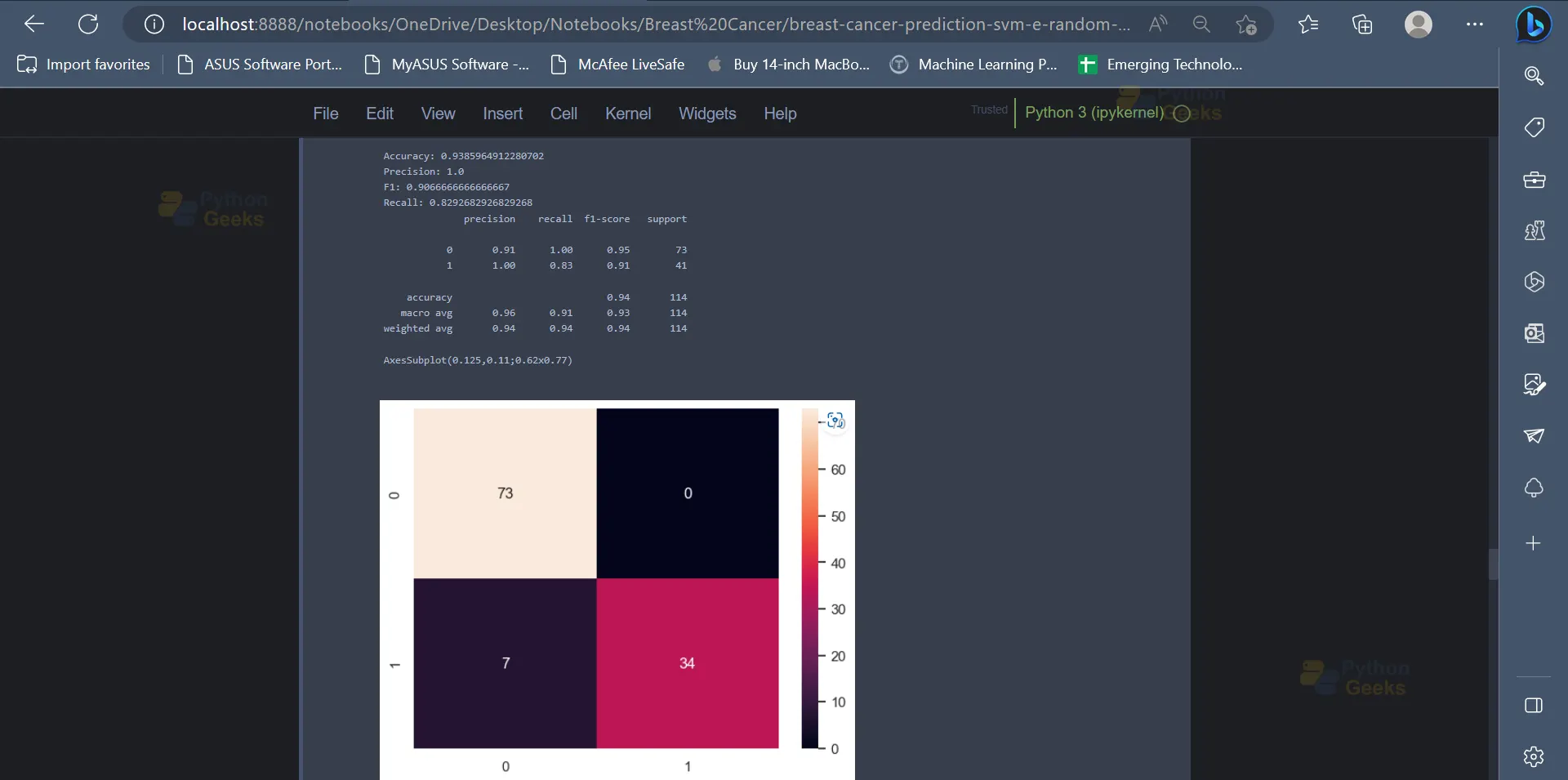
The performance of the model can be tested using metrics like accuracy score, precision, recall, confusion matrix etc. Logistic regression provides an accuracy of 93.85% on the dataset.

from sklearn.metrics import confusion_matrix, accuracy_score, precision_score, f1_score, recall_score, classification_report
print('Accuracy:',accuracy_score(y_test, y_pred))
print('Precision:',precision_score(y_test, y_pred))
print('F1:',f1_score(y_test, y_pred))
print('Recall:',recall_score(y_test, y_pred))
print(classification_report(y_test, y_pred))
print(sns.heatmap(confusion_matrix(y_test, y_pred), annot=True))

Output

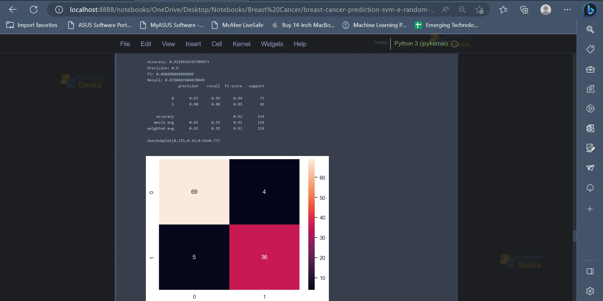
14. The next model which we will be using is the Decision Tree Classifier. On analysing the metrics it can be seen that the Decision Tree Classifier provides an accuracy of 92.1% on the dataset.

from sklearn.tree import DecisionTreeClassifier
model = DecisionTreeClassifier(criterion='entropy',class_weight='balanced',random_state=123)
model.fit(X_train, y_train)
y_pred = model.predict(X_test)


print('Accuracy:',accuracy_score(y_test, y_pred))
print('Precision:',precision_score(y_test, y_pred))
print('F1:',f1_score(y_test, y_pred))
print('Recall:',recall_score(y_test, y_pred))
print(classification_report(y_test, y_pred))
print(sns.heatmap(confusion_matrix(y_test, y_pred), annot=True))

Output

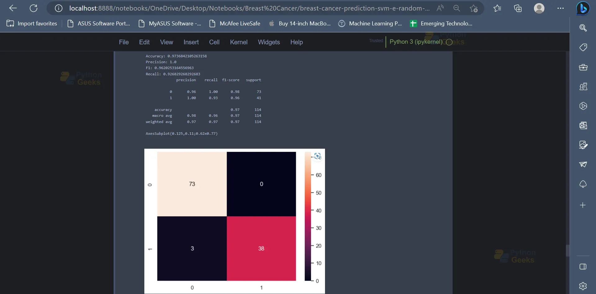
15. Moving forward, we will be implementing the Support Vector Machine Classifier in order to classify the data points. The SVM Classifier has an accuracy of 97.36% on the dataset.

from sklearn.svm import SVC
model = SVC(kernel='poly', class_weight='balanced',random_state=123)
model.fit(X_train, y_train)
y_pred = model.predict(X_test)


print('Accuracy:',accuracy_score(y_test, y_pred))
print('Precision:',precision_score(y_test, y_pred))
print('F1:',f1_score(y_test, y_pred))
print('Recall:',recall_score(y_test, y_pred))
print(classification_report(y_test, y_pred))
print(sns.heatmap(confusion_matrix(y_test, y_pred), annot=True))

Output

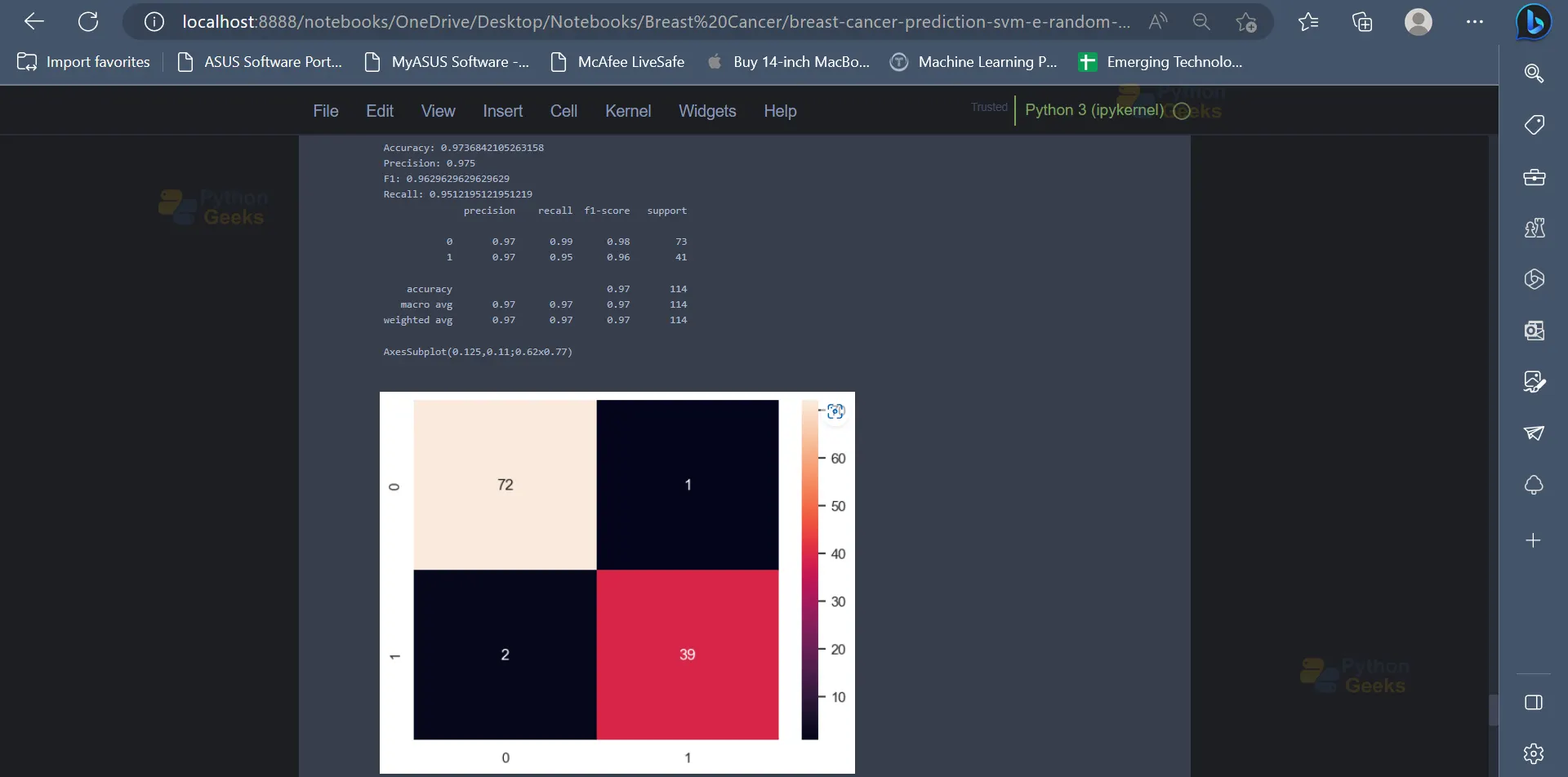
16. Next up, the Random Forest algorithm can be used to classify the data points into their respective classes or categories. Similar to the previous model, the Random Forest Algorithm has an accuracy of 97.36% on the dataset.

from sklearn.ensemble import RandomForestClassifier
model = RandomForestClassifier(n_estimators=500, max_depth=3,random_state=123)
model.fit(X_train, y_train)
y_pred = model.predict(X_test)


print('Accuracy:',accuracy_score(y_test, y_pred))
print('Precision:',precision_score(y_test, y_pred))
print('F1:',f1_score(y_test, y_pred))
print('Recall:',recall_score(y_test, y_pred))
print(classification_report(y_test, y_pred))
print(sns.heatmap(confusion_matrix(y_test, y_pred), annot=True))

Output

Conclusion

In conclusion, the development of personalised treatment regimens for patients and the improvement of diagnostic accuracy have both been demonstrated by the categorization of breast cancer using machine learning approaches. Large datasets can include patterns and relationships that may not be immediately apparent to human specialists. These patterns and relationships can be found using techniques like decision trees and support vector machines. This may lead to better patient outcomes and has the potential to hasten the discovery of novel breast cancer therapies. Future studies in this area are required to enhance these methods and broaden their use to more varied patient groups.