Gradient Boosting Algorithm in Machine Learning

In this article, we will discuss one of the most trending algorithms that we use for prediction in Machine Learning- Gradient Boosting. It is more commonly known as the Gradient Boosting Machine or GBM. It is one of the most widely used techniques when we have to develop predictive models.

In this article from PythonGeeks, we will discuss the basics of boosting and the origin of boosting algorithms. We will also look at the working of the gradient boosting algorithm along with the loss function, weak learners, and additive models. Towards the end of the article, we will look at some of the methods to improve the performance over base algorithm along with various regularization schemes. So, let’s look at the introduction of Boosting.

Introduction to Boosting

While learning about the various Machine Learning models, you might have heard a lot about the term Boosting. According to some researchers, it is one of the most misinterpreted terms in the discipline of Machine Learning. The aim of the algorithm lies in developing a first-hand model structure based on the training dataset. Then, we tend to develop the second model to resolve the drawbacks of the previous model. Let us try to understand this definition with the help of an example.

Consider a model where you have to train it with the help of n data points, and the result of this model is one of the two classes 0 and 1. Now, our aim is to develop a model that will predict the class of the new test data that we feed into the algorithm. After this, we randomly select from the training dataset and give it as an input to the first model M1. Along with this, we proceed further with the assumption that all the weights have the same weight in the beginning.

Since M1 is a weak learner, there is a high possibility of misclassification of some of the training data. Now we observe the misclassified data and modify its weight to rectify the error when we will pass it to the next model M2. We iterate this process with all other models till we are left with the least possible error or almost perfectly predicted data. In such a way, the new data points will have to go through all the weak learners to predict accurate results.

Introduction to Gradient Boosting Algorithm

The main base of the Gradient Boosting Algorithm is the Boosting Algorithm working. The algorithm focuses upon developing a sequential structure of models that try to reduce the errors of the previous models. But the major question that we have to tackle is how are we going to achieve this? How are we going to reduce the errors of the consequent models? We can achieve this by rectifying the results of the residuals of the previous models.

The type of Gradient Boosting Algorithm that we use depends on the type of problem we need to tackle. We deploy the Gradient Boosting Regressor when we have to deal with a continuous column and the Gradient Boosting Classifier when we have to use it for classification problems. The sole difference between these two problems is the use of “loss function”. The main focus of the algorithm is to minimize the loss function in order by repetitively adding weak learners through the gradient descent.

We can boost the accuracy of a predictive model in two ways:

a. By embracing feature engineering or

b. Applying boosting algorithms straight away.

Purpose of Gradient Boosting

Gradient Boosting tends to train many models in a gradual, additive, and sequential manner. The primary difference between AdaBoost and Gradient Boosting Algorithm is the way in which the two algorithms identify the shortcomings of weak learners (in this case decision trees). While the AdaBoost model explores the shortcomings by making use of high weight data points, gradient boosting tends to perform the same by using gradients in the loss function (y=ax+b+e, e needs a special mention as it is the error term). The loss function accounts to be a measure indicating how good are model’s coefficients are at performing fitting the underlying data. A logical understanding of loss function would be directly interlinked with what we are trying to optimize.

History of Boosting Algorithm

The idea behind the development of Boosting Algorithm arose with the thesis of whether we can add a series of weak learners in order to manifest better results from them.

Michael Kearns stated that a weak learner could be thought of as the one whose performance rate is a bit better than any randomly chosen chance.

Here, the main basis of the development was hypothesis boosting. It was the idea that worked on filtering observations, then developing more weak learners in order to handle the queries that the first weak learners could not handle.

Adaboost- The First Grafient Model

The first realization of boosting that witnessed great success in the application was Adaptive Boosting or AdaBoost for the shorter version. The weak learners that we can identify in the working of AdaBoost are decision trees with a single split. These splits are known as decision stumps for their shortness.

AdaBoost tends to work by weighting the observations, emphasizing more weight on difficult to classify instances and less on those weights that the algorithm has already handled well. The algorithm tends to add new weak learners sequentially that have their focus on their training on the more difficult patterns.

The algorithm tends to make predictions by the majority vote of the weak learners’ predictions, which the algorithm weighs by their individual accuracy. The most widespread form of the AdaBoost algorithm was for binary classification problems and was known by the name of AdaBoost.M1.

Generalization of AdaBoost as Gradient Boosting

AdaBoost and related algorithms were amongst the first algorithms that were recast in a statistical framework first by Breiman and coined the term ARCing algorithms for them. This framework was further enhanced by Friedman and the term coined for these was Gradient Boosting Machines. Later the algorithms were just called gradient boosting or gradient tree boosting.

This class of algorithms categorized themselves as a stage-wise additive model. This took place due to the fact that the algorithm adds one new weak learner at a time and tends to freeze existing weak learners in the model and left unchanged.

The generalization enabled arbitrary differentiable loss functions for their usefulness, broadening the technique beyond binary classification problems in order to support regression, multi-class classification, and more.

Working of Gradient Boosting Algorithm

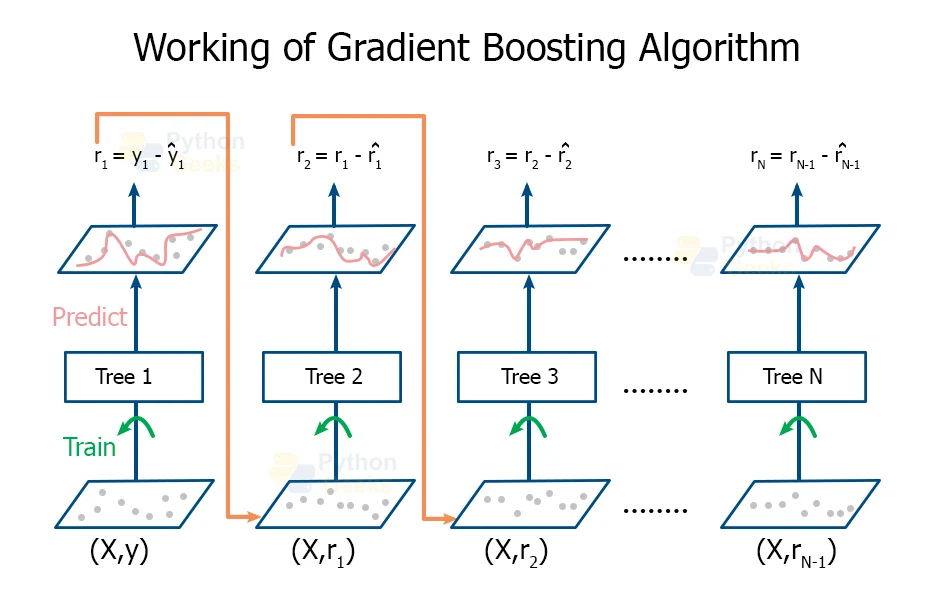
The working of the Gradient Boosting Algorithm can be divided on the basis of its major three elements:

Optimizing the loss function
Fabricating a weak learner for predictions
Development of an additive model of weak learners to minimize the loss function

1. Loss Function

The loss function that we use for the models, depends on the type of algorithm that we are using. The main focus of selecting any loss function is that the loss function should be differentiable. There are many standard functions available for usage, but one can define their own loss function depending on the type of problem they tackle.

As an example, we can use a squared error in the case of regression problems whereas we use a logarithmic loss in the case of the classification problem.

The most beneficial feature of using a gradient boosting framework is that we do not need to derive a new boosting algorithm for each loss function that we use while solving the problem. As an alternative, the gradient boosting algorithm is generic enough so that we can use any differentiable loss function along with the algorithm.

2. Weak Learner

We use decision trees as weak learners while using the gradient boosting algorithm. We precisely use the regression trees whose outputs are real values for splits and we can add the outputs together, to allow subsequent models to add their outputs with the “correct” residual in the predictions.

Also, we construct these trees using the greedy algorithm by choosing the best split points that are based on the purity scores like Gini or those who can minimize the loss function.

In the beginning, especially in the AdaBoost, we used very short decision trees that only had a single split. These splits were known as decision stumps. We can also develop larger trees with the general leveling of 4 to 8 levels.
This technique makes sure that the learners remain weak throughout the algorithm but we can still construct them in a greedy manner.

3. Additive Model

We add the new trees one at a time in the model such that the pre-existing trees remain unaltered. We tend to follow the gradient descent procedure in order to minimize the loss while adding the trees.

Conventionally, developers used gradient descent in order to minimize a set of parameters like the coefficients in the regression equations or the weights associated with the nodes of the neural networks. After the calculation of the errors or the loss, we modify the weights to minimize the error.

In gradient descent, we have weak learning sub-models or more precisely the decision trees. After we calculate the loss, we need to add a new tree to perform the gradient descent to reduce the loss. We can achieve this by adding parameters to the new trees. We then modify these parameters of the tree and move the tree in the right direction by reducing the residual loss.

This procedure is functional gradient descent.

Implementation of Gradient Boosting Regressor

Gradient Boosting for Classification

#PythonGeeks Code for Boosting Classification
#evaluate gradient boosting algorithm for classification
from numpy import mean
from numpy import std
from sklearn.datasets import make_classification
from sklearn.model_selection import cross_val_score
from sklearn.model_selection import RepeatedStratifiedKFold
from sklearn.ensemble import GradientBoostingClassifier
# define dataset
X, y = make_classification(n_samples=1000, n_features=20, n_informative=15, n_redundant=5, random_state=7)
# define the model
model = GradientBoostingClassifier()
# define the evaluation method
cv = RepeatedStratifiedKFold(n_splits=10, n_repeats=3, random_state=1)
# evaluate the model on the dataset
n_scores = cross_val_score(model, X, y, scoring='accuracy', cv=cv, n_jobs=-1)
# report performance
print('Mean Accuracy: %.3f (%.3f)' % (mean(n_scores), std(n_scores)))

The above code will have the output as

Mean Accuracy: 0.898 (0.031)

# make predictions using gradient boosting for classification
from sklearn.datasets import make_classification
from sklearn.ensemble import GradientBoostingClassifier
# define dataset
X, y = make_classification(n_samples=1000, n_features=20, n_informative=15, n_redundant=5, random_state=7)
# define the model
model = GradientBoostingClassifier()
# fit the model on the whole dataset
model.fit(X, y)
# make a single prediction
row = [0.2929949, -4.21223056, -1.288332, -2.17849815, -0.64527665, 2.58097719, 0.28422388, -7.1827928, -1.91211104, 2.73729512, 0.81395695, 3.96973717, -2.66939799, 3.34692332, 4.19791821, 0.99990998, -0.30201875, -4.43170633, -2.82646737, 0.44916808]
yhat = model.predict([row])
# summarize prediction
print('Predicted Class: %d' % yhat[0])

The output of the above code will depict the results as

Predicted Class: 1

Gradient Boosting for Regression

#PythonGeeks code for Gradient Boosting for Regression
from numpy import mean
from numpy import std
from sklearn.datasets import make_regression
from sklearn.model_selection import cross_val_score
from sklearn.model_selection import RepeatedKFold
from sklearn.ensemble import GradientBoostingRegressor
# define dataset
X, y = make_regression(n_samples=1000, n_features=20, n_informative=15, noise=0.1, random_state=7)
# define the model
model = GradientBoostingRegressor()
# define the evaluation procedure
cv = RepeatedKFold(n_splits=10, n_repeats=3, random_state=1)
# evaluate the model
n_scores = cross_val_score(model, X, y, scoring='neg_mean_absolute_error', cv=cv, n_jobs=-1)
# report performance
print('MAE: %.3f (%.3f)' % (mean(n_scores), std(n_scores)))

The above code will depict the output as

MAE: -62.461 (3.253)

# gradient boosting ensemble for making predictions for regression
from sklearn.datasets import make_regression
from sklearn.ensemble import GradientBoostingRegressor
# define dataset
X, y = make_regression(n_samples=1000, n_features=20, n_informative=15, noise=0.1, random_state=7)
# define the model
model = GradientBoostingRegressor()
# fit the model on the whole dataset
model.fit(X, y)
# make a single prediction
row = [0.20543991, -0.97049844, -0.81403429, -0.23842689, -0.60704084, -0.48541492, 0.53113006, 2.01834338, -0.90745243, -1.85859731, -1.02334791, -0.6877744, 0.60984819, -0.70630121, -1.29161497, 1.32385441, 1.42150747, 1.26567231, 2.56569098, -0.11154792]
yhat = model.predict([row])
# summarize prediction
print('Prediction: %d' % yhat[0])

The code output will depict the value as

Prediction: 37

Improvements to Basic Gradient Boosting

Gradient Boosting is an example of a greedy algorithm and it can overfit any training dataset speedily.

We can maximize the benefits of the algorithm by regularization methods. These methods can then penalize the parts of the algorithm that can lead to the maximization of the loss function. We perform this in order to enhance the performance of the algorithm since it reduces the chances of overfitting.

In the following section, we will discuss the 4 enhancements that we can perform to improve the gradient boosting algorithm

Tree Constraints
Shrinkage
Random Sampling
Penalized Learning

1. Tree Constraints

The most important factor that we have to consider while developing the gradient boosting model is to make sure that learners remain weak even after gaining skills.

There are a number of ways in which we can constrain the trees in the gradient descent. Below are some of the constraints that we can impose on the trees

We have to keep checking the number of trees that we add to the model. When we add more trees to the model, then the overfitting will occur quite slowly. The advisable factor remains that we keep adding trees to the model until we stop observing further progress.

The depth of the trees also plays an important role in the performance of the model. The deeper the tree, the more complex the algorithm will get. We always prefer to use trees that have 4 to 8 levels to achieve accurate results.

As the depth of the tree, the number of nodes or leaves on the trees is also a crucial factor in deciding the performance of the model. Though the size of the model is affected by the change in the number of nodes, we can neglect this constraint if other constraints are also present.

Before we consider any split to train the data for prediction, we need to observe the number of observations at each split.

The main constraint that we need to observe is the possibility of minimum loss while adding new nodes to the tree.

2. Weighted Updates

We need to add the prediction of each tree in a sequential manner. We can slow down the learning of the model by considering the contribution of each tree to the sum of all the outputs. This addition of the weights is called shrinkage of a learning rate.

The weights of the shrinkage can slow down the learning rate of the model. It then results in a situation in which we have to add more trees to the model. This in turn results in the delay in the training period of the model which results in the configuration trade-off between the rate of addition of trees and the learning rate.

3. Stochastic Gradient Boosting

The biggest insight in the training and adding of the random forests was that we allowed the greedy creation of trees from the subsamples of the training of the dataset.

We can use this same benefit to reduce the correlation between the trees in the sequential structures of the gradient boosting algorithm. This variation in the boosting of the sequence is the stochastic gradient boosting.

A few variants of stochastic boosting are:

Subsampling rows before the creation of each tree
Subsampling columns before the creation of each tree
And Subsampling columns before consideration of the splits

4. Penalized Gradient Boosting

We can add more constraints to the parameterized trees along with the constraints of their structure. Instead of using the conventional decision trees like CART as weak learners, we tend to use a modified form called a regression tree. These regression trees have numeric values in the nodes of the trees. In some of the writings, these values of the leaves are written as weights of the trees.

We can regularize the leaf weights by using popular regularization functions like:

L1 regularization of the weights
L2 regularization of the weights

Conclusion

With this, we have reached the end of the article that dealt with the Gradient Boosting Algorithm. In this PythonGeeks article, we came to know about one of the most important prediction algorithms- the Gradient Boosting Algorithm. We came across the history and work of the gradient boosting algorithm. Towards the end, we also saw some of the improved methods for the performance of the algorithm. Hope that this article gives you a thorough understanding of the Gradient Boosting Algorithm.