Gaussian Mixture Model in Machine Learning

Gaussian Mixture Model or more commonly known as, the Mixture of Gaussian, is not so much of a model at its core as it is basically a probability distribution. It is a universally used model for generative unsupervised learning or clustering algorithms. It is also known by the name Expectation-Maximization Clustering or EM Clustering and follows the optimization strategy.

We make use of the Gaussian Mixture models for representing Normally Distributed subpopulations within an overall population. The major advantage of using Mixture models is that they do not require knowing beforehand which subpopulation a data point belongs to. It consents the model to learn the subpopulations automatically on its own. This constitutes a form of unsupervised learning and classifies the model under it.

Due to its immense popularity and use, it is necessary for us to know about this algorithm and its implementation in greater depth. Due to this, PythonGeeks brings to you, an article that will guide you through the hooks and crooks of this topic. We will cover topics like Gaussian Distribution, Gaussian Mixture Model, and implementation. Apart from this, we will look at the applications and their comparison with other models. Towards the end, we will discuss a case study concerned with GMM. So, without further ado, let us dive into the introduction part and get to know about the Gaussian Distribution.

What is Gaussian Distribution?

Gaussian is a kind of distribution, and it is amongst the most popular and mathematically convenient types of distribution. At its core, distribution is a listing of all the outcomes of an experiment and the probability associated with each one of the outcomes.

A Gaussian distribution is a kind of distribution where half of the data distributes itself on the left of it, and the other half of the data distributes itself on the right of it. It requires an evenly distributed dataset, and one can observe just by the thought of it intuitively how mathematically convenient it makes the problems.

So, the actual question that arises here is, why do we need to define a Gaussian or Normal Distribution? We require a mean, which is the average of all the data points. That will define the center of the curve and the standard deviation which will demonstrate how spread out the data is.

We can certainly consider Gaussian distribution as a great distribution to model the data in such cases where the data reaches a peak and then decreases accordingly. In similar circumstances, in Multi Gaussian Distribution, we ought to have multiple peaks with multiple means and multiple standard deviations.

The mathematical formulation of Gaussian distribution using the mean and the standard deviation called the Probability Density Function is:

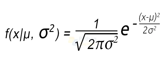
This equation depicts a function of a continuous random variable for which the integral across an interval gives the probability that the value of the variable lies within the equivalent interval.

Introduction to Gaussian Mixture Model

In certain instances, our data may have multiple distributions or it may have multiple peaks. It does not necessarily always have one peak, and one can observe that by looking at the data set. It will appear like there are multiple peaks arising here and there. There exists two peak points and the data seems to be moving up and down twice or maybe three times to four times. However, if there are Multiple Gaussian distributions that can demonstrate this data, then we can build the so-called Gaussian Mixture Model.

In other words, we can convey that, if we have three Gaussian Distribution namely, GD1, GD2, GD3 having mean as µ1, µ2, µ3 and variance σ1, σ2, σ3, then for a given set of data points GMM will try to identify the probability of each data point fitting to each of these distributions.

It is a probability distribution that comprises multiple probability distributions and consists of Multiple Gaussians.

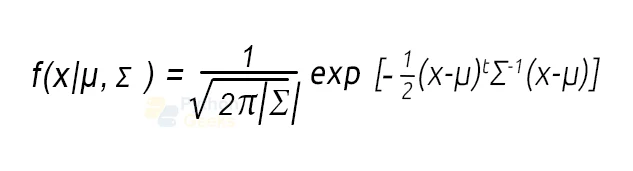
We may define the probability distribution function of d-dimensions Gaussian Distribution as:

Why do we use Gaussian Mixture Model?

Now, one might think that despite having powerful algorithms like K-means and Gradient Descent, why should we look forward to working with the Gaussian Mixture Model. Well, the answer is quite simple, because of the drawbacks of these models. In the following section, we will discuss how these models have certain drawbacks and limitations that we need to be aware of.

Comparison with K-Means

Let us consider some income-expenditure examples that we need to visualize using these algorithms. The k-means algorithm seems to be working pretty well with such examples. However, if you observe closely, you will notice that all the clusters that the algorithm creates have a circular shape. This happens because the algorithm updates the centroids of the clusters iteratively using the mean value.

For difference, consider the following example where the distribution of points is not possible in a circular form. What do you think will the algorithm results if we use k-means clustering on this data? It would still try to group the data points in a circular fashion. This attempt certainly proves to be a hindrance and defies the purpose of using K-Means.

As a consequence of which, we require a different way to assign clusters to the data points. So as an alternative to using a distance-based model, we may now use a distribution-based model. And that is where Gaussian Mixture Models will help us achieve our goal!

Comparison with Gradient Descent

Gradient descent tends to compute the derivative which shows us the direction in which the data wants to move in or in what direction should we move the data of the parameter of our model such that the function of our model is optimized enough to fit our data.

However, what if we are not able to compute a gradient of a variable, implying we are not able to compute a derivative of a random variable. The Gaussian mixture model needs to have a random variable. It is a stochastic model implying it is non-deterministic. We are not able to compute the derivative of a random variable stating the exact reason why we cannot use gradient descent.

Expectation Maximization

Expectation-Maximization (EM) is a statistical algorithm that we can employ for finding the right model parameters. We typically make use of the EM when the data has missing values, or in simple words, when our dataset is incomplete. These missing variables are referred to as latent variables. We then consider the target, or cluster number, to be unknown when we tend to be working on an unsupervised learning problem.

Given that we do not have the values for these latent variables, Expectation-Maximization tends to use the existing data to determine the optimum values for these variables and then tries to find the model parameters. On the basis of these model parameters, we tend to go back and update the values for these latent variables, and the algorithm proceeds to deliver an accurate result.

Broadly, the Expectation-Maximization algorithm has two steps for these value predictions:

1. E-step: In this step, the algorithm makes use of the available data to estimate (predict) the values of the missing variables.

2. M-step: On the basis of the estimated values generated in the E-step, the algorithm makes use of the complete data to update the parameters.

Usage of E-M

1. We can use E-M to fill in missing data.

2. It is quite helpful in finding the values of latent variables.

The disadvantage of the EM algorithm is that it has a slow convergence rate and it converges barely up to the local optima only.

Implementation of Gaussian Mixture Model in Python

#PythonGeeks code for the implementation of Gaussian Mixture Model
 
#Importing the necessary datasets
import numpy as np 
import pandas as pd 
import matplotlib.pyplot as plt 
from pandas import DataFrame 
from sklearn import datasets 
from sklearn.mixture import GaussianMixture 
  
# loading the iris dataset 
iris = datasets.load_iris()  
# selecting first two columns  
X = iris.data[:, :2]   
# turning it into a dataframe 
d = pd.DataFrame(X) 
# ploting the data 
plt.scatter(d[0], d[1])
gmm = GaussianMixture(n_components = 3)  
# Fit the GMM model for the dataset  
# which expresses the dataset as a  
# mixture of 3 Gaussian Distribution 
gmm.fit(d)  
# Assigning a label to each sample 
labels = gmm.predict(d) 
d['labels']= labels 
d0 = d[d['labels']== 0] 
d1 = d[d['labels']== 1] 
d2 = d[d['labels']== 2] 
plt.show() 
 
# ploting three clusters in same plot 
plt.scatter(d0[0], d0[1], c ='r') 
plt.scatter(d1[0], d1[1], c ='yellow') 
plt.scatter(d2[0], d2[1], c ='g')
plt.show() 

The output for the following GMM code will be

Next, we will print the converged log-likelihood values

# printing the converged log-likelihood value
print("The mean:",gmm.means_)
print('\n')
print("The covariance matrix:",gmm.covariances_) 
print("The converged log-likelihood value:",gmm.lower_bound_) 
# print the number of iterations needed 
# for the log-likelihood value to converge 
print("The number of iterations needed for the log-likelihood value to converge:",gmm.n_iter_)

The output of the code for the likelihood values is

The mean: [[6.68055626 3.02849627]
 [5.01507898 3.4514463 ]
 [5.9009976  2.74387546]]


The covariance matrix: [[[0.36153508 0.05159664]
  [0.05159664 0.08927917]]

 [[0.11944714 0.08835648]
  [0.08835648 0.11893388]]

 [[0.27671149 0.08897036]
  [0.08897036 0.09389206]]]
The converged log-likelihood value: -1.4987505566235162
The number of iterations needed for the log-likelihood value to converge: 8

Applications of GMM

1. GMM is extensively used in the field of signal processing.

2. GMM stipulates good results in language Identification.

3. Customer Churn is another example of the broad usage of GMM.

4. GMM finds itself useful in Anomaly Detection.

5. We can even use GMM to track the object in a video frame.

6. Apart from these, GMM also finds its usage in the classification of songs based on genres.

The Segmentation of Homogenous Bacterial Colony – Case Study in Gaussian Mixture Model

Recognition of images in digital images in the areas where homogeneous data was recurring, as was in the case of research conducted to cluster homogeneous bacterial colonies for the purpose of their size estimation. The isolation of the bacterial culture regions from the dish was achieved with the help of image segmentation. The researchers parametrized this histogram with the help of the Gaussian Mixture Model using the Expectation Minimization.

With the help of this algorithm, the researchers could achieve a good level of grey color distribution and were also able to merge separate distributions of two different objects.

Conclusion

With this, we have successfully concluded the article that guided us through the basic tutorial of the GMM. In this article, we came across the topics of Gaussian Distribution and the Gaussian Mixture Model. We even came across the drawbacks of other algorithms and even the implementation of GMM in Python. Towards the end, we came across a case study involving the usage of GMM in the Segmentation of Homogenous Bacterial Colonies. Hope, that this article from PythonGeeks was able to counter all your queries regarding Gaussian Mixture Model.