Dimensionality Reduction in Machine Learning

Have you ever tried to study the data that we feed into the Machine Learning algorithms to process? Unlike the data that we consider for learning the concepts of Machine Learning, the data that we use for the training of the Machine Learning Model is quite complex. For our simplicity, we try to understand the data that is much simpler to handle and has fewer dimensions. However, the data that we feed to the models is quite large and complex since it has a resemblance to real-world entities. Because of this reason, this data has more dimensions and has more dimensions associated with it.

In this article from PythonGeeks, we bring to you a technique that Machines use to minimize these dimensions of the data- Dimensionality Reduction. In this article, we will talk about the basics of the Dimensionality Reduction technique, its components, and various methods for the reduction of the data dimensions. We will also cover the importance, features, advantages, and disadvantages of dimensionality reduction. So, let’s look at the introduction of Dimensionality Reduction.

Problem with many Inputs

The performance of machine learning algorithms is affected drastically by too many input variables.

If we represent our data using rows and columns, such as in a spreadsheet, then the input variables are the columns that we feed in as input to a model to predict the target variable. These input variables are also called features.

We can imagine these columns of data representing dimensions on an n-dimensional feature space along with the rows of data as points in that space. It is a very useful geometrical interpretation of a dataset.

Having numerous dimensions in the feature space can mean that the volume concerning that particular space is very large, and thus, the points that we have in that space (rows of data) often depict a small and non-representative sample.

These factors can drastically impact the performance of machine learning algorithms fit on data with many input features. We generally refer to this phenomenon as the “curse of dimensionality”. We can thus conclude that having too many input variables can lead to a less precise output.

Introduction to Dimensionality Reduction

Till now, we have seen that we are able to train Machine Learning models on real-life data in order to process it to perform tasks like prediction, classification, and image processing. However, it becomes quite troublesome to train these models to attain accurate results since the data that we encounter in real-life has more dimensions associated with it. We have to consider all of these features in order to classify them accurately. We call these classifying features variables.

The more the number of these features, the harder it gets to train our dataset and acquire accurate results. But many times, some of these features are correlated to each other, and this makes it redundant to consider them for classification.

Apart from these issues, we also encounter data, where the sensors may generate some redundant features leading to an increase in the complexity of the problem. This is where Dimensionality Reduction comes to our rescue. It mainly focuses on transforming a large dataset containing vast dimensions into a dataset with lesser dimensions without losing the purpose of the dataset. We perform dimensionality reduction on Machine Learning models in order to make training the model an easier task and get accurate results.

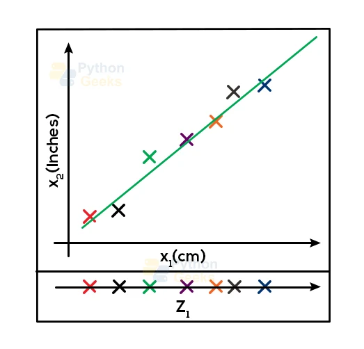
For a better understanding of this, let us look at the following examples. Here, we consider a huge dataset containing two features x1 and x2. In this dataset, x1 is the measure of a particular piece of object in cm whereas x2 is the measure of the same object in inches. Now, as we observe from the figure, both the features convey the same meaning which is the length of the object.

Furthermore, if we use this dataset to train the machine learning model, then both the features would look similar to the model causing confusion. This will induce a lot of noise in the system. Therefore, it is better to use just one dimension to gain better results. So, we transform this 2D data (having features x1 and x2) into a 1D dataset (having feature z1).

We can attain similar results in other larger datasets as well. With the help of dimensionality reduction, we can obtain the same results that we can get using larger datasets.

Motivation

• When we consider data that we acquire from real-life problems, the data is comparatively quite large and has higher dimensions.
• In these high-dimensional data, it becomes quite troublesome to process the data. It sometimes becomes necessary to reduce the dimensions of the data without changing its meaning.
• Though sometimes we can process this larger data, it is always advisable to reduce the dimensions of the data for better results.

Components of Dimensionality Reduction

While performing dimensionality reduction on larger datasets, we have to consider these two components:

Feature Selection

In this component, we need to look for a subset of the actual set of the variables of the dataset. We even need to find a subset that we can use to model the problem. There are usually three ways to do so. They are Filter, Wrapper, and Embedded.

Feature Extraction

In this component, we tend to reduce the data of higher-dimensional space into the data of lower-dimensional space. In other words, it tends to reduce the number of dimensions of the data.

Methods for Dimensionality Reduction

The various methods that we can use for dimensionality reduction are

• Principal Component Analysis (PCA)
• Linear Discriminant Analysis (LDA)
• Generalized Discriminant Analysis (GDA)

We can use the above-mentioned methods for linear as well as non-linear reduction depending on the method that we are using. PCA is one of the widely used Dimensionality Reduction methods.

Importance of Dimensionality Reduction

Lately, the problem of the increase in redundant dimensions of the datasets is closely interlinked to the fixation of recording the data at a granular layer than it was in the conventional methods. However, this is not a problem that we are facing recently. It so happens that due to the increase in data in recent times, the problem of redundant dimensionality has been highlighted significantly.

We are storing a large amount of data in recent times with the help of transponders and sensors. These sensors record data on a continuous basis and store it for future processing. However, due to the surge in the usage of sensors, there is a significant increase in redundant features. Apart from this, there are many examples where we can observe the redundancy of features in the recorded dataset. Some of these examples are enlisted below:

• Casinos track their customer movements with the help of cameras.
• Capturing of public data by political parties in order to increase their reach on the field.
• Set-top box collecting information about your preferences in your type of entertainment.

With the increase in such data, the redundancy in the collected data increases manifoldly. Due to these reasons, it becomes necessary for the developers to dimensionally reduce the dataset to effectively train the machine learning model.

Methods to Perform Dimensionality Reduction

Though there are many methods through which we can effectively perform dimensionality reduction on the dataset, we have curated a list of the top methods that we use for dimensionality reduction.

1. Missing Values

You may have encountered problems where the dataset that you collected has some missing data points. In such situations, we may consider one of these two approaches. First, we may tend to observe the dataset carefully and analyze the reason for the missing value and drop this variable with an accurate method. Second, we may encounter a situation where we have too many missing data points. In this case, imputing the missing value is more complex than dropping the variable.

Here, we tend to act on the second case. The main reason behind this is the unaltered data due to the dropping of the variable. In situations where the missing data point does not contain much data, we can drop this variable.

2. Low Variance

Let us assume a dataset in which we have a variable with a constant value (it has a similar value for all data points of the variable). In such cases, these data points act as redundant branches for the dataset. Dropping such variables may alter the variance of data. However, in the case of higher-dimensional data, we can drop such constant data points from the dataset since it does not have much effect on the dataset.

3. Decision Tree

This is one of the most effective dimensionality reduction techniques. It can tackle multiple challenges like missing values, outliers, and identifying significant variables.

4. Random Forest

Random Forest works in a similar fashion as a decision tree. The only drawback for this type of dimensionality reduction is that the algorithm is biased towards variables that have a greater number of distinct values.

5. High Correlation

Dimensions that have a higher correlation may tend to lower the efficiency of the model. Apart from this, it is also not advisable to have multiple variables containing the same information. This is also known as “Multicollinearity”.

6. Manifold Learning

We can make use of the techniques from high-dimensionality statistics for dimensionality reduction. These techniques are sometimes referred to as “manifold learning” and we can use them to fabricate a low-dimensional projection of high-dimensional data, in order to make data visualization precise and less complex.

We design the projection in such a way so that both create a low-dimensional representation of the dataset while best preserving the salient structure or relationships within the data.

7. Backward Feature Elimination

In this type of dimensionality reduction, we generally consider all the dimensions of the dataset. Then we try to compute the sum of squares of errors (SSR) after we eliminate each of the variables. Then we observe the change caused by the removal of these variables over the SSR and identify those variables who have caused the least change. We are then left with a dataset containing one less variable as compared to the original one. We then tend to iterate the same process till we are left with no variables that we can drop.

8. Autoencoder Method

We can also use Deep learning neural networks to perform dimensionality reduction.
A popular approach towards constructing these networks is autoencoders. The technique involves framing a self-supervised learning problem where a model must reproduce the input precisely.

9. Matrix Factorization

We can use the techniques from linear algebra for dimensionality reduction as well. Particularly, we make use of the matrix factorization methods to reduce a dataset matrix into its constituent elements. Examples, where we implement this reduction technique, include the eigendecomposition and singular value decomposition.

10. Factor Analysis

In such types of reductions, we deal with data points containing some correlation with other data points. Here, we group together the data points having correlation making them a single entity. This makes the data have a lesser number of points as compared to the original dataset. There are two methods that we can use to perform factor analysis on these grouped factors: EFA (Exploratory Factor Analysis) and CFA (Confirmatory Factor Analysis).

11. Principal Component Analysis

In this technique, we try to linearly combine the original variables to transform them into a set of new variables. These newly transformed sets of variables are known as Principal Components. We form these principal components in such a way that each newly formed component accounts for most of the variations of the dataset that we can originally observe in the actual dataset. This results in the highest possible variance for the dataset.

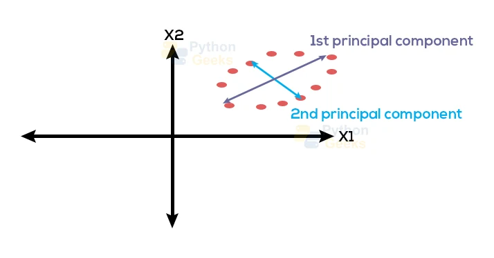
The second principal dataset is arranged orthogonally to the first principal component. In simple words, the second principal component tends to cover the variance of the dataset that the first principal component was unable to cover. For a dataset having two dimensions, we can develop a PCA model containing only two principal components. We should always try to standardize the variables before applying PCA since it is highly sensitive to measurements.

Algorithms for Dimensionality Reduction

1. Decomposition Algorithm

Decomposition algorithm in scikit-learn comprises dimensionality reduction algorithms. We can invoke various techniques of this library by using the following command:

from sklearn.decomposition import PCA, KernelPCA, NMF

2. Singular Value Decomposition

The singular value decomposition or, more commonly referred to as SVD is a factorization method of a real or complex matrix. It is efficient when we are working with a sparse dataset; a dataset having numerous zero entries. We generally find This type of dataset in the Recommender Systems, rating, and reviews dataset, and so.

Tips for Dimensionality Reduction

There is no definite rule for dimensionality reduction and no mapping of techniques to such problems.

Instead of abiding by the same system, the best approach is to use systematic controlled experiments to discover what dimensionality reduction techniques, when paired with your model of choice, will result in the best performance on your dataset.

Typically, it is observed that linear algebra and manifold learning methods assume that all input features have the same scale or distribution. This gives an implication that it is a good practice to either normalize or standardize our data set prior to using these methods if the input variables have different scales or units.

Dimensionality Reduction Tools and Libraries

Due to its wide applications in a variety of algorithms, many libraries support the implementation of dimensionality reduction. Amongst the many libraries, the most popular library for dimensionality reduction is scikit-learn (sklearn). This library consists of three main modules that are beneficial for dimensionality reduction algorithms:

1. Decomposition algorithms

• Principal Component Analysis
• Kernel Principal Component Analysis
• Non-Negative Matrix Factorization
• Singular Value Decomposition

2. Manifold learning algorithms

• t-Distributed Stochastic Neighbor Embedding
• Spectral Embedding
• Locally Linear Embedding

3. Discriminant Analysis

• Linear Discriminant Analysis

Feature Selection in Reduction

While performing dimensionality reduction, the main concern lies in the selection of the features that are redundant and retaining the useful ones. In order to tackle this problem, below are some criteria to select the variables:

• We can apply a Greedy algorithm to add or remove variables till it satisfies a certain criterion.
• We can make use of shrinking and penalizing methods which will add costs to the datasets for carrying too many functions.
• Filtering out variables on the basis of correlation.

Advantages of Dimensionality Reduction

• Dimensionality Reduction is a great tool when it comes to data compression and acquiring lesser data space.
• It significantly decreases computational time.
• If the datasets contain redundant features, then dimensionality reduction gets rid of them easily.
• It helps in faster processing of the same dataset with reduced features.
• It also handles multicollinearity which improves the performance of the overall algorithm.
• Reducing the dimensionality of the data helps in the precise visualization of the data. With more visualization of the data, we can conveniently lookout for errors.
• Since it reduces redundant features of the dataset, it consequently reduces the noise corrupting the data.

Disadvantages of Dimensionality Reduction

• Even though we are careful while reducing the data, we may still end up with significant data loss.
• While applying PCA, the algorithm tends to look for a linear correlation between the data points, which is not required in some cases.
• Apart from these, we may not accurately judge the number of Principal Components that we need for the reduction.

Applications of Dimensionality Reduction

As we have seen throughout the articles, Dimensionality Reduction helps us in making models that are reliable and accurate. Because of these reasons, this technique finds its way in various applications like:

• Customer relationship management
• Text categorization
• Image retrieval
• Intrusion detection
• Medical image segmentation

Conclusion

With this, we have reached the end of the Dimensionality Reduction article from PythonGeeks. In this article, we tried to cover some of the basics of the Dimensionality Reduction technique. We came across the various features affecting the reduction. We also saw why dimensionality reduction is so important and looked at some of the examples of the reduction method. Hope that this article was able to deliver all the information that you needed for Dimensionality Reduction.