31 Deep Learning Key Terms You Must Know

Have you ever encountered difficulty while learning Machine Learning or Deep Learning tutorials? Do you ever feel that even though the article claims that it is trying to convey the topic in the easiest of ways and yet you cannot grasp the concept properly? This might happen because of your lack of experience with the usage of Machine Learning terms. You might sometimes feel that some of the terms that the article you are reading uses require citations for a better understanding.

PythonGeeks brings to you a well-defined glossary of the widely used key terms in the Machine Learning and Deep Learning discipline. So, let’s start our article to get the brief of these terms.

Deep Learning Key Terms and Terminologies

1. Activation Function

In the training of neural networks, we pass the input in the form of a linear component. We then tend to add a nonlinear function to these linear components. We achieve this by applying the activation function to the bias-added input.

The main focus of the activation function is to traverse the linear input combination to the output layer effectively. If we denote the activation layer by f(), then the non-linear combination that we feed to the output layer will look like f(a*w1+b), where, a is the input, w1 is the weight associated with the node, and b is the bias.

2. Artificial Neural Network

 Many developers consider Artificial Neural networks or simply Neural networks to be the backbone of the Deep Learning discipline. The basic structure of the ANN comprises closely interlinked neurons that imitate the behavior of the biological neurons.

The objective of forming neural networks is to have near to similar imitation of human thinking in the machine training models. The neurons of the Neural Network have weights and biases associated with them, which update themselves during the process. These are then passed to a nonlinear activation function to achieve a desired output from the output layer.

3. Backpropagation

This term is associated with neural network models like ANN, CNN, and RNN. Whenever we think about the training of these models, we think about the weights and biases that we assign to the nodes of the model. We also tend to look out for errors at the end of iteration of each process of information processing. In general terms, we pass the input to the input layer and expect output from the output layer.

However, backpropagation deals with the reversal of this data flow. In backpropagation, as soon as we receive the output at the output layer, we calculate the error related to the output by comparing the difference between the actual output and the expected output. The model then passes this error through the loop and we adjust the weights and biases of the network in order to minimize the error. This process of updating the weights and biases using the gradient of the cost function is backpropagation. The data flow in backpropagation is from the output layer to the input layer.

4. Batches

While training the neural networks with trained data, there are two ways in which we can feed the input to the network. In the first method, we pass the input data to one for the neural network for processing. While doing this, the processing speed reduces and the model may not process efficiently.

In the other method, instead of feeding a whole lot of data in one round, we tend to break the data into batches of equal-sized chunks in a random fashion. These chunks are the batches in which we feed the data. This makes the model more efficient and speedier.

5. Batch Normalization

We can understand the concept of batch normalization with a simple analogy of the working of dams. At any river, dams act as a checkpoint for the flow of the river water. Similarly, batch normalization acts as a dam for the data flow for the neural network. It makes sure that the data distribution at each layer of the network is similar to the previous layer.

In the process of training the neural model, the weights associated with the node update itself. Due to this, the subsequent layer receives differently-shaped data. However, the subsequent expects the data similar to the preceding layer. Therefore, we have to explicitly normalize the training data in order to ensure a smooth training process.

6. Bias

We know that the nodes in the neural network associated with them help with the data flow. Apart from these weights, we have to augment one more linear entity to the nodes- Biases. In the flow of the data, we deal with the multiplication of the weights of the nodes. We add the weights to these multiplied weights in order to increase their range. After this addition, the final linear input component looks like a*w1+bias.

7. Cost Function

When we are training the neural model, the main aim of the model is to predict the output of the new data as close as possible to the expected output based on the trained data. We measure this precision of the output with the help of the cost function. The major aim of the cost function is to reprimand the model in case of an error. Thus, our aim focus shifts to intensifying the accuracy while minimizing the error. Minimization of the error deals with minimizing this cost function. The learning process thus concentrates on minimizing the cost function.

8. Convolutional Neural Network (CNN)

Convolutional Neural Networks is a Neural Network that deals with image processing and classification. Normal neural networks lack the ability to work with image processing. The complexities of processing the image increase significantly with the increase in the size of the image making the neural networks inefficient to work with.

Convolutional Neural Networks tend to “convolve” these images for better processing. In other words, CNN tries to reduce the number of parameters associated with the image. The CNN tries to pass the input image over various filters which try to convert the input volume of the image into 2-dimensional activation maps. The stacked network of these activation maps makes it effective to work with image-related inputs.

9. Data Augmentation

Data Augmentation deals with the increment of the new data that we derive from the given input data. We perform these additions in order to enhance the accuracy of the prediction results.

For a better understanding let us consider an example of a dull image of a cat. Now, if we improve the brightness of the image, then the training model might benefit from this adjustment and give better results. By brightening the image, we are trying to improve the quality of the image. As another example, consider the image below. Slightly tilting the image provides us with a better view of the image. This enhancement is known as Data Augmentation.

10. Dropout

As you might have guessed from the name, Dropout is a regularization technique that omits certain neurons of the hidden layer in order to produce a reliable result. This technique helps to avoid over-fitting during the training of the model. While the data flow from one layer to the other with the help of neurons, the main processing results depend on the geometry in which these neurons are arranged.

Dropping out some of the neurons results in the change of the output. We combine the various results that we acquire by the different orientations of the neurons. This helps in achieving reliable outputs.

11. Epochs

The iteration of a single data flow process during the training of the model of all batches including forward and backpropagation is an epoch. Simply, one epoch is the single passage of forward and backpropagation of a whole lot of the input data.  You can modify the number of epochs that you need for training the entire input data. Using a larger number of epochs may result in a high precision output, however, it will also require an increased training period. 

12. Exploding Gradient Problem

This gradient problem is the polar opposite of the Vanishing Gradient Problem. Unlike the latter, the Exploding Gradient Problems renders a high gradient to the activation function. While we perform backpropagation on the neural model, this problem renders a high weight to one of the neurons of the networks, making the effect of other neurons insignificant. We can tackle this problem with the help of clipping the gradient. By clipping the gradient to avoid the weights from reaching a certain value, the weights remain uniform.

13. Filters

Filters in Convolutional Neural Networks are analogous to weights in other neural networks. We multiply these filters with the voluminous information of the image in order to generate a convoluted image. First, we create a filter with smaller dimensions as compared to the input image. We then multiply these filters to various sections of the image to create the convoluted output. During the process, the filter values update themselves in the same way as weights update themselves in backpropagation for cost minimization.

14. Forward Propagation

In general terms, the data flow in any neural network follows the same path. We first feed the data to the input layer which then traverses to the hidden layers which then further traverses to the output layer. The data flow of these layers is generally unidirectional without any loops. This data restrictedly flows in the forward direction. This means the data will pass from the input layer to the output through the hidden layers only. This traversal is Forward Propagation.

15. Gradient Descent

Gradient Descent is an optimization algorithm, which means that we can use gradient descent when we need to minimize the cost function of the neural network.

To understand this in a better way, let us consider the analogy of climbing down the hills. We always focus on taking small steps while descending the hills, so that we don’t apparently fall while crossing. We follow a similar approach while finding the minimized cost function of the network. Also we consider proportionally negative portions of the gradients in order to locate the local minima of the cost function.

16. Input/ Output/ Hidden Layers

The basic structure of any neural network model comprises these layers. As the name defines their purposes, we make use of the input layer to feed in the data to the neural model. The output layer generates the output and acts as the final stage of the processing. The intermediate layers are the hidden layers.

The main processing of the training like prediction, classification, regression takes place at these layers. While the input and output layers are visible to the developer, the intermediate layers do not disclose their working and hence are called “hidden”.

17. Learning Rate

Learning rate is the minimization of the cost function that we encounter while the iteration of the data flows from the input layer to the output layer. It is the measure of how fast we approach the minima of the cost function.

The main challenge associated with the learning rate is the choice of learning rate. We should not choose a higher learning rate because we can miss the optimization point in that case. On the other hand, the learning rate should not be too low as it will take a comparatively larger period to complete the process.

18. Multilayer Perceptron (MLP)

As we know, the neural network models tend to replicate the functioning of the biological neural network with the help of artificial neurons. However, a single neuron is incapable of producing accurate results. Therefore, we use a stacked layer of these neurons in order to obtain accurate results.

Generally, we deal with the input layer, the hidden layers, and the output layers. These layers comprise multiple neurons along with their neurons are connected to the neurons of other layers as well.

19. Network Layers

Network layers are the building blocks of any Neural Network. The stacking of these layers is what forms the main structure of the neural networks. Different layers perform significantly different functions of the neural network. A layer defines an operation like taking in the input, processing it, and traversing it further. The main network layers that we encounter while training the neural networks are the input layer, hidden layers, and output layers.

20. Neuron

Similar to the biological neural network, the artificial neural network is also made up of neurons. We can think of neurons as the fundamental processing units of neural networks. The main function of these neurons is to take in the input data, process it, and transmit the output to other neurons or transmit the processed data as the final output. 

21. Padding

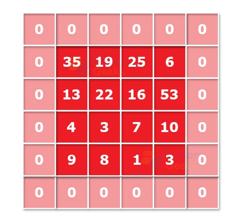
While processing the image input with the help of a Convolutional Neural Network, we tend to reduce the dimensionality of the image. In order to have an output image of the same dimension as that of the input image, we add a layer of zeroes to the processed image. This process of adding an extra layer of zeroes is padding.

After padding, the convulsed image has the same size as that of the actual image. In valid padding, the process tends to retain the actual or “valid” pixels of images as intact as possible.

22. Pooling

Pooling is generally done in an attempt to avoid over-fitting. In the structure of CNN, we periodically augment pooling layers to reduce the number of parameters associated with the image. There are various pooling operations like max-pooling or average pooling that we use to attain the desired results. However, the most efficient pooling technique is to have a pooling layer of filter size (2,2) using the MAX pooling.

23. Recurrent Neuron

Recurrent neurons function in the same way as the Recurrent Neural Network. Here, we send the output of the neuron back to the input layer for t timestamps. You can think of this neuron as a series of different neurons at various time intervals whose output is sent back to the input for t iterations. The motive behind doing this is to achieve more generalized output from the neurons.

25. Recurrent Neural Network

As we have seen earlier, RNN is a beneficial neural network when we have to deal with sequential data in which the prediction of the subsequent output is predicted using the previous output. Unlike other networks, RNN has loops associated with them. These loops are advantageous since they help in storing the output of the previous iteration and thus accurately predict the succeeding pattern.

Like the working of the recurrent neuron, the output of one iteration of the process is again sent to the input layer for t timestamps. If we encounter any error during the process, then we tackle it using backpropagation. It is also known as backpropagation through time (BTT).

26. ReLu

ReLu is the acronym for Rectified Linear Units along it is a type of activation function. The main advantage of using ReLu over sigmoid functions is that it works well on hidden layers. The mathematical representation of the function: f(x)= max(x,0)

The function returns the value of X if X>0 or it returns 0 if X<=0. The major use of this function is that it has a constant derivative value which helps in faster training of the network.

27. Sigmoid

Sigmoid is by far one of the most commonly used activation functions for the training of neural networks. It outputs a much smoother range of values that lie between 0 and 1. This helps us in observing the changes that occur in the output with the slightest of changes in the input. The activation function is

Sigmoid(x) = 1/(1+e-x)

28. Softmax

The generalized use of the softmax activation function is in the output layer of the classification problems. It works in the same fashion as that of the sigmoid function. The only difference lies in the way this function optimizes the output to the sum up to 1.

Though the sigmoid function is capable of handling classification problems, it fails to deliver accurate results in the case of multiclass classification. Softmax function effectively handles this by assigning each class with the values to easily interpret the probabilities.

29. Training

The term training is often associated with the “learning” of the neural network. In simple terms, training is the process of taking in the input, processing it, and acquiring the output. We then compare the acquired output with our expected output and send the data again to the input layer with a slight change in the weights of the nodes. Training of models helps us in gaining better outputs.

30. Vanishing Gradient Problem

Unlike the Exploding gradient problem, the Vanishing Gradient problem arises when the activation function is too small. During backpropagation, the multiplication of these low activation functions may lead the neurons to become insignificant. This causes some of the neurons to “vanish” from the network. Because of this, the neural network may forget its long-range dependency. This problem generally arises with Recurrent Neural Networks.

31. Weights

As we have seen many times now, each node of the neural network associates itself with a weight. When we pass the input to the neural network, we multiply the input with this associated weight. Thus, we then have a weight associated with the neurons as well. We determine the importance of any node on the basis of the weight associated with them.

In the beginning, all the nodes have similar weights which then update themselves during the training process. The higher the importance of the neuron, the higher its weight will be. If a node has zero weight associated with it, then we can consider it to be insignificant.

Conclusion

With this, we have reached the end of the glossary. Being unaware of these might lead you to trouble while learning about deep learning. This article from PythonGeeks will act as your go-to guide whenever you feel that you are unable to understand the concepts of Deep Learning. Though the vocabulary of any technology is vast, we have curated the most important terms for you.