Credit Card Fraud Detection using Machine Learning

This project aims to build a machine learning model to detect credit card fraud. The dataset used in this project is the “creditcard.csv” file which contains credit card transactions made in September 2013 by European cardholders. The data set contains a total of 284,807 transactions, out of which 492 transactions are fraudulent. The class distribution in the dataset is highly imbalanced, with the majority class being non-fraudulent transactions. To address this class imbalance, the minority class is oversampled using the RandomOverSampler technique. After oversampling, the features are scaled using the StandardScaler.

A Logistic Regression model is then trained using GridSearchCV to optimize hyperparameters. The model’s performance is evaluated using metrics such as the confusion matrix, classification report, and ROC curve. Finally, the confusion matrix is plotted using seaborn to visualize the model’s performance.

What is Credit Card Fraud Detection?

Credit card fraud detection is the process of identifying and preventing fraudulent transactions made using credit cards. Fraudulent transactions occur when a person or entity uses stolen or fraudulent credit card information to make purchases or obtain funds. Credit card fraud can result in significant financial losses for both the individuals whose credit card information was stolen and the financial institutions that issued the cards. Fraud detection systems use various algorithms and techniques to detect fraudulent transactions and prevent them from being processed, protecting consumers and financial institutions from financial losses.

About Dataset

The dataset used for this classification problem is ‘creditcard.csv’. The dataset contains transactions made by credit cards in September 2013 by European cardholders. The dataset has 31 columns and 284,807 rows. The ‘Class’ column is the target variable, where 1 means fraud and 0 means not fraud.

Prerequisites for Credit Card Fraud Detection Using Machine Learning

1) Pandas
2) Seaborn
3) Matplotlib
4) Scikit-learn
5) Imblearn

Download Machine Learning Credit Card Fraud Detection Project

Please download the source code of Machine Learning Credit Card Fraud Detection Project from the following link: Machine Learning Credit Card Fraud Detection Project Code.

Steps to Develop Credit Card Fraud Classifier in Machine Learning

The code executes the following steps to develop the credit card fraud classifier in machine learning:

1) Importing the required libraries
2) Reading the dataset
3) Exploratory data analysis
4) Splitting the dataset into features and labels
5) Oversampling the minority class using RandomOverSampler
6) Scaling the features using StandardScaler
7) Splitting the resampled dataset into training and testing sets
8) Creating the logistic regression model
9) Setting up the GridSearchCV to optimize hyperparameters
10) Training the model
11) Predicting the labels for the testing set
12) Evaluating the model performance by printing the confusion matrix, classification report, and accuracy score
13) Plotting the ROC curve
14) Plotting the confusion matrix

1. Importing the required libraries

import pandas as pd
import seaborn as sns
import matplotlib.pyplot as plt
from sklearn.preprocessing import StandardScaler
from sklearn.model_selection import train_test_split, GridSearchCV
from sklearn.linear_model import LogisticRegression
from sklearn.metrics import confusion_matrix, classification_report, roc_curve, roc_auc_score
from imblearn.over_sampling import RandomOverSampler

The first section of the code imports the necessary Python libraries for data pre-processing, visualization, model building, and evaluation. These libraries include Pandas, Seaborn, Matplotlib, Scikit-learn, and Imbalanced-learn.

2. Reading the dataset

data = pd.read_csv('creditcard.csv')

This code reads in the credit card dataset from a CSV file using Pandas.

3. Exploratory data analysis

print(data.head())
print(data.describe())
print(data.info())

This section prints some basic statistics about the dataset, such as the first few rows, summary statistics, and information about the columns.

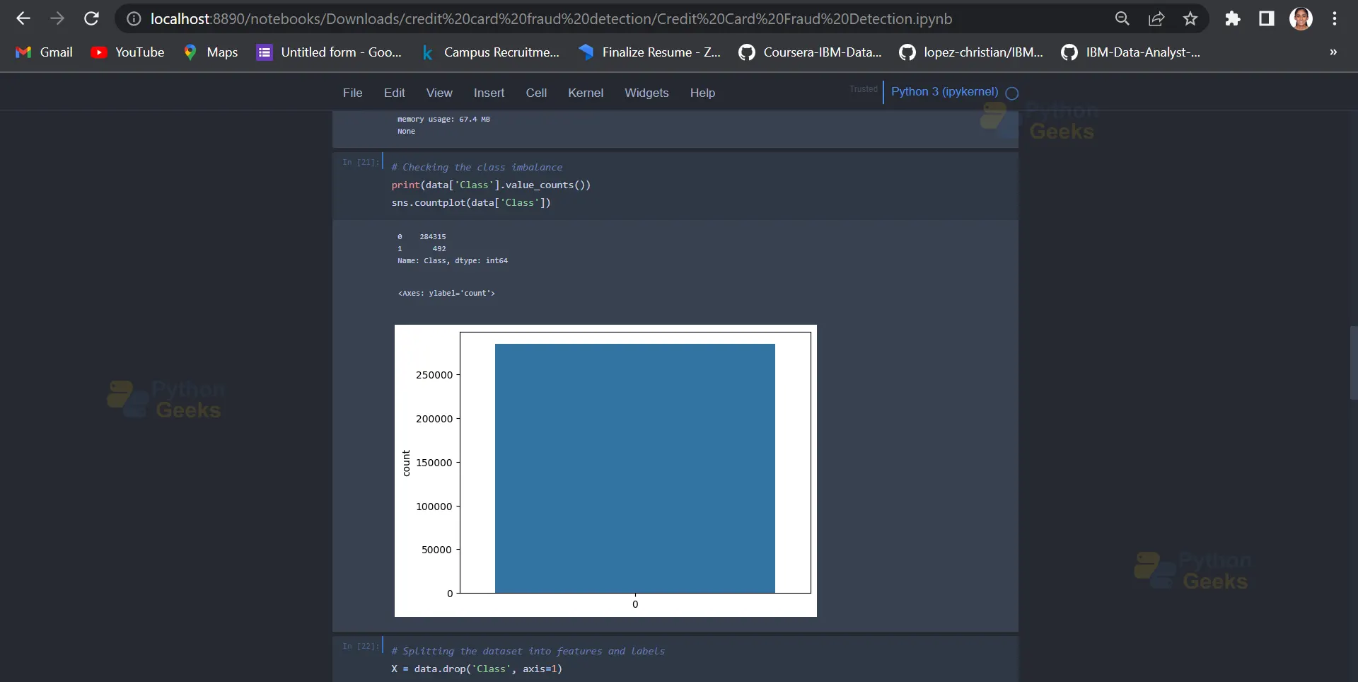
The below code checks the class imbalance of the target variable, ‘Class’. The first line prints out the count of each class value (0 for non-fraudulent and 1 for fraudulent transactions), while the second line creates a countplot using Seaborn to visualize the class distribution.

print(data['Class'].value_counts())
sns.countplot(data['Class'])

Output:

4. Splitting the dataset into features and labels

X = data.drop('Class', axis=1)
y = data['Class']

This code splits the dataset into the features (X) and the target variable (y) by dropping the ‘Class’ column from the original dataset to create X and assigning the ‘Class’ column to y.

5. Oversampling the minority class using RandomOverSampler

oversampler = RandomOverSampler()
X_resampled, y_resampled = oversampler.fit_resample(X, y)

This code uses the RandomOverSampler function from the Imbalanced-learn library to oversample the minority class (fraudulent transactions) to balance the class distribution in the dataset. This is done to improve the performance of the logistic regression model.

6. Scaling the features using StandardScaler

scaler = StandardScaler()
X_resampled = scaler.fit_transform(X_resampled)

This code scales the features in the dataset using the StandardScaler function from Scikit-learn to standardize the features to have a mean of 0 and a standard deviation of 1.

7. Splitting the resampled dataset into training and testing sets

X_train, X_test, y_train, y_test = train_test_split(X_resampled, y_resampled, test_size=0.3, random_state=42)

This code splits the oversampled dataset into training and testing sets using the train_test_split function from Scikit-learn. The test_size parameter is set to 0.3 to allocate 30% of the data for testing, and random_state is set to 42 to ensure reproducibility.

8. Creating the logistic regression model

logistic = LogisticRegression()

This code creates an instance of the logistic regression model from Scikit-learn.

9. Setting up the GridSearchCV to optimize hyperparameters

params = {'C': [0.001, 0.01, 0.1, 1, 10, 100], 'penalty': ['l1', 'l2']}
grid_search = GridSearchCV(logistic, params, cv=5)

This line sets up the hyperparameter grid to be searched. In this case, the grid is set to contain 6 different values for the regularization parameter C, and 2 different penalty functions (l1 and l2). The code also sets up the GridSearchCV object with the logistic regression model and the parameter grid. The cv parameter specifies the number of folds in the cross-validation.

10. Training the model

grid_search.fit(X_train, y_train)

This line fits the GridSearchCV object to the training data, using the parameter grid to search for the best combination of hyperparameters.

11. Predicting the labels for the testing set

y_pred = grid_search.predict(X_test)

This line uses the fitted GridSearchCV object to predict the class labels of the testing data.

12. Evaluating the model performance by printing the confusion matrix, classification report, and accuracy score

confusion = confusion_matrix(y_test, y_pred)
print("Confusion matrix:\n", confusion)
report = classification_report(y_test, y_pred)
print("Classification report:\n", report)
accuracy = grid_search.score(X_test, y_test)
print(f"Accuracy: {accuracy:.2%}")

Output:

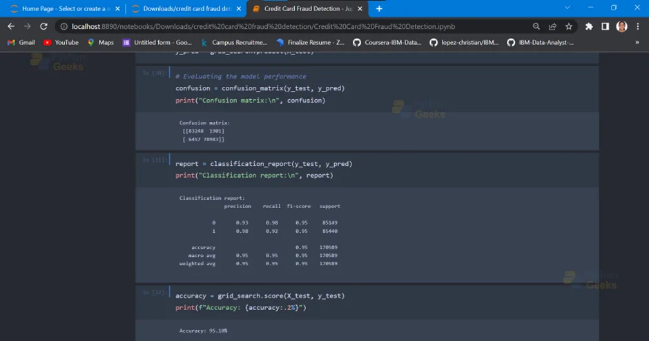
Therefore, the model has an accuracy of 95.10%.

13. Plotting the ROC curve

y_prob = grid_search.predict_proba(X_test)[:,1]
fpr, tpr, thresholds = roc_curve(y_test, y_prob)
auc = roc_auc_score(y_test, y_prob)
plt.plot(fpr, tpr, label=f"ROC curve (area = {auc:.2f})")
plt.plot([0, 1], [0, 1], 'k--')
plt.xlabel('False Positive Rate')
plt.ylabel('True Positive Rate')
plt.title('Receiver Operating Characteristic (ROC) Curve')
plt.legend()

This code plots the Receiver Operating Characteristic (ROC) curve for the model’s predictions, showing the trade-off between true positive rate and false positive rate. The area under the curve (AUC) is also calculated and displayed in the plot.

Output:

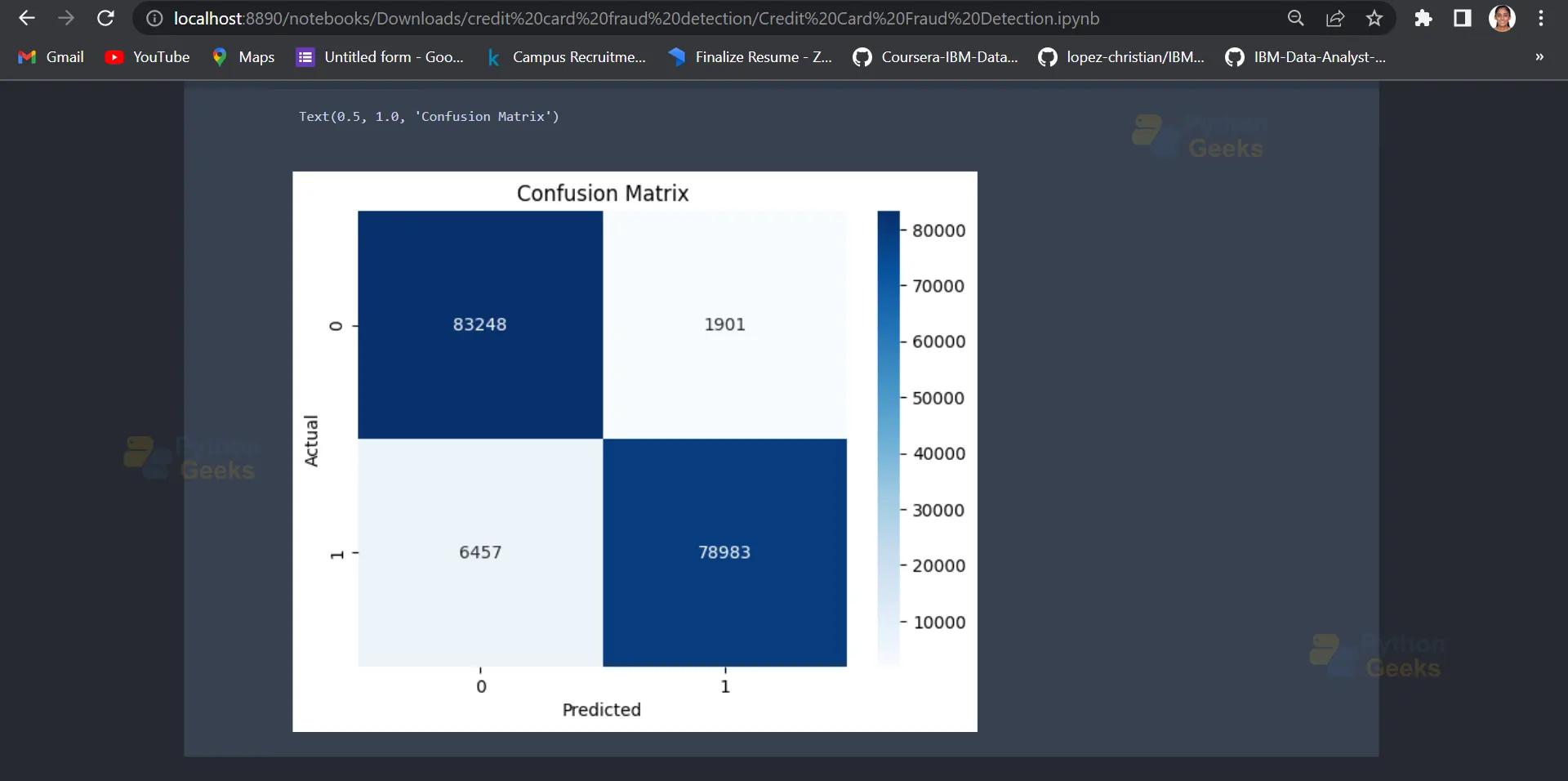
14. Plotting the confusion matrix

sns.heatmap(confusion, cmap='Blues', annot=True, fmt='g')
plt.xlabel('Predicted')
plt.ylabel('Actual')
plt.title('Confusion Matrix')

Output:

Summary

The code develops a credit card fraud classifier using logistic regression and evaluates its performance using the confusion matrix, classification report, and ROC curve. The code also addresses the class imbalance issue in the dataset by oversampling the minority class using RandomOverSampler.