Classification in Machine Learning

Machine learning is a domain that largely deals with studies and mainly focuses on algorithms that learn from examples. On the other hand, Classification is a task that needs the use of machine learning algorithms that train how to assign a class label to the sample dataset from the problem domain. A go-to example of this is classifying emails as spam.

There are numerous different types of classification tasks that you may encounter in the vast arena of machine learning. Apart from them, you may also encounter the specialized approaches to modeling that you may use for each one of them.

PythonGeeks brings to you, this tutorial, that will discover different types of classification predictive modeling in machine learning. We will try to cover the basics of classifications in a detailed and comprehensive way. We will discuss topics like the evaluation of classifiers, classification models, and classification predictive modeling. Towards the end, we will discuss the four main types of classifications in Machine Learning along with their codes and output. Therefore, let us look at the introduction of classification.

What is Classification in Machine Learning?

We can simply define Classification as the process of recognition, understanding, and grouping of objects and ideas into preset categories or sub-populations within a large group. With the assistance of these pre-categorized training datasets, classification in machine learning programs leverages a vast range of algorithms to classify future datasets into respective and relevant categories for simplification.

Classification algorithms that we use in machine learning utilize input training data for the function of predicting the similarities or probability that the data that follows will come under one of the predetermined categories. One of the most familiar applications of classification is for filtering emails as spam or non-spam.

To put it simply, classification is a form of pattern recognition technique in Machine Learning. In the present context, classification algorithms that we apply to the train data tend to find the same pattern in future new data sets.

Learners in Classification Problems

We generally encounter two types of Learners in the classification problems. They are:

1. Lazy Learners: Lazy Learner stores the training dataset as the preliminary step and waits until it receives the test dataset. In the Lazy learner case, the algorithm performs classification on the basis of the most related data stored in the training dataset. It requires less time in training but more time for predictions. Examples of this type of learner are K-means and Case-Based reasoning

2. Eager Learners: Eager Learners tend to develop a classification model on the basis of a training dataset before receiving a test dataset. Unlike Lazy learners, Eager Learner requires more time in learning and less time in prediction. Examples of this type of learner are Decision Tree and ANN.

Evaluating Classifiers in Machine Learning

To analyze the accuracy of our classifier model, we need some accuracy measures for comparison. We make use of the following methods to analyze how well our classifiers are predicting:

1. Holdout Method: It is amongst one of the most common methods of analyzing the accuracy of our classifiers model. In this method, we tend to divide the data into two sets, namely, a training set and a testing set. We show the training set to our model, and the model learns from the data present in it.

The data present in the testing set is denied from the model, and after we train the model, we use the testing set to test its accuracy. The training set will have both the features as well as the corresponding label. However, the testing set will only comprise the features and the model will have to predict the corresponding label.

2. Bias and Variance: We can define Bias as the difference between our actual and predicted values of the model. Bias is the straightforward assumption that our model tends to make about our data to be capable of predicting new data. It directly corresponds to the patterns recognized in our data. When the Bias of our data is high, the assumptions that our model makes are too basic, the model is not able to capture the important features of our data. This phenomenon is called underfitting.

3. Precision and Recall: We make use of Precision to calculate the model’s ability to classify values accurately. We can denote it by dividing the number of accurately classified data points by the total number of classified data points for that class label present in our dataset.

Evaluating Classification Models

As soon as our model is ready, we need to test it for its accuracy and performance. Be it a regression model or a classification model, each model requires evaluation before deploying it in the market. For classification models, we have the following methods of evaluation.

1. Log Loss or Cross Entropy Loss

We make use of it for evaluating the performance of a classifier, for which the output is a probability value between 0 and 1. For an accurate binary Classification model, the value of log loss should converge to 0. The value of log loss tends to increase if the predicted value deviates from the actual value. The lower log loss indicates the higher accuracy of the model.

2. Confusion Matrix

The confusion matrix facilitates us with a matrix/table as output and demonstrates the performance of the model. We can even refer to it as the error matrix. The matrix comprises predictions result in a summarized form, which has a total number of correct predictions and incorrect predictions from the training model.

3. AUC-ROC Curve

ROC curve is the acronym for Receiver Operating Characteristics Curve whereas AUC is the acronym for Area Under the Curve. It is a graph that depicts the performance of the classification model at different thresholds. In an attempt to visualize the performance of the multi-class classification model, we tend to use the AUC-ROC Curve. We plot the ROC curve against TPR and FPR, where TPR (True Positive Rate) is on the Y-axis whereas FPR(False Positive Rate) is on the X-axis.

Classification Models in Machine Learning

The major algorithms that we use as the classification models for our classification problems are:

1. Naive Bayes: It is a classification algorithm that makes the assumption that predictors in a dataset are independent of the dataset. This indicates that it assumes the features are completely unrelated to each other. As an example, for a given banana, the classifier will see that the fruit is yellow in color, has an oblong shape, and is long and tapered. All of these features will tend to contribute independently to the probability of it being a banana and these features are not dependent on each other.

2. Decision Tree: It is an algorithm that we use to visually represent decision-making regarding the given dataset. We can make a Decision Tree by asking a yes/no question and dividing the answer to lead to another decision. The deciding question is present at the node and it places the resulting decisions below at the leaves.

3. K-Nearest Neighbor: KNN is a classification and prediction algorithm that we can use to divide data into classes on the basis of the distance between the data points. K-Nearest Neighbor makes the assumption that data points which are close to one another must be similar and as a consequence of that, the data point that we classify will be grouped with the closest cluster.

Use Cases of Classification Models

Some of the extensively used cases of Classification models are:

• Email Spam Detection
• Speech Recognition
• Identifications of Cancer tumor cells.
• Drugs Classification
• Biometric Identification

Classification Predictive Modeling

In machine learning, classification signifies a predictive modeling problem where we predict a class label for a given example of input data.

From a modeling point of view, classification needs a training dataset with numerous examples of inputs and outputs from which it learns.

A model will make use of the training dataset and will calculate how to accurately map examples of input data to specific class labels. As such, the training dataset must be sufficient enough to represent the problem and have many examples of each class label.

There are various different types of classification algorithms for modeling classification predictive modeling problems.

There is no definite theory on how to map algorithms onto the given problem types. However, it is generally recommended that a practitioner makes use of controlled experiments and analyze themselves about which algorithm and algorithm configuration will result in the best performance for a given classification task.

We evaluate Classification predictive modeling algorithms on the basis of their results. Classification accuracy is a major metric that we use to evaluate the performance of a model on the basis of the predicted class labels. Classification accuracy is not accurate but is a good starting point for many classification tasks.

1. Binary Classification

We use Binary Classification for those classification tasks that have two class labels.

Examples for binary classification include:

• Email spam detection.
• Churn prediction
• Conversion prediction

On a general basis, a binary classification task comprises one class that is the normal state and another class that is the abnormal state.

We allocate the class for the normal state as the class label of 0 and the class with the abnormal state as the class label of 1.

It is usual to model a binary classification task with a model that predicts a Bernoulli probability distribution for each example that we feed to the model.

As we have seen earlier, the Bernoulli distribution is a discrete probability distribution that spans over a case where an event will have a binary outcome as either a 0 or 1. For classification, this indicates that the model predicts a probability of an example belonging to class 1 or the abnormal state.

Popular algorithms that we can use for binary classification include:

• Logistic Regression
• k-Nearest Neighbors
• Decision Trees
• Support Vector Machine
• Naive Bayes

The code for binary classification is

# PythonGeeks example for binary classification task
from numpy import where
from collections import Counter
from sklearn.datasets import make_blobs
from matplotlib import pyplot
# Now we need to define dataset
X, y = make_blobs(n_samples=1000, centers=2, random_state=1)
# Next, summarize dataset shape
print(X.shape, y.shape)
# Further, summarize observations by class label
counter = Counter(y)
print(counter)
#Next, summarize first few examples
for i in range(10):
  print(X[i], y[i])
# for visualization,plot the dataset and color the by class label
for label, _ in counter.items():
  row_ix = where(y == label)[0]
  pyplot.scatter(X[row_ix, 0], X[row_ix, 1], label=str(label))
pyplot.legend()
pyplot.show()

The following code for Binary Classification will give the output as

2. Multi-Label Classification

This algorithm refers to those classification tasks that consist of two or more class labels, in which one or more class labels may predict for each example.

To understand it better, consider the example of a photo classification. Here, a given photo may have multiple objects present in the scene and a model may predict the presence of multiple known objects in the photo, such as bicycle, apple, person, cat, dog, and so on.

Unlike binary classification and multi-class classification, where the model predicts a single class label for each example.

It is usual to model multi-label classification tasks with a model that predicts multiple outputs, with every output taking the prediction as a Bernoulli probability distribution. This is significantly a model that makes multiple binary classification predictions for each example of the dataset.

The code for the execution of Multi-Line Classification is

# PythonGeeks example of a multi-label classification task
from sklearn.datasets import make_multilabel_classification
# define dataset
X, y = make_multilabel_classification(n_samples=10000, n_features=3, n_classes=2, n_labels=2, random_state=1)
# summarize dataset shape
print(X.shape, y.shape)
# summarize first few examples
for i in range(10):
  print(X[i], y[i])

The output of the following Multi-label class classification code will be:

3. Multi-Class Classification

Unlike binary classification, multi-class classification does not consist of the notion of normal and abnormal outcomes. Instead, we classify examples as belonging to one among a range of known classes.

The number of class labels may be very huge on some problems. For example, a model may predict a photo as belonging to one among thousands or tens of thousands of faces in a face recognition system that we build using the classification model.

Problems that involve the prediction of a sequence of words, such as text translation problems, we may also consider a special type of multi-class classification. Every word in the sequence of words that the model predicts involves a multi-class classification where the size of the vocabulary demonstrates the number of possible classes that the model may predict and could be tens or hundreds of thousands of words in size.

The Python code for Multi-Class Classification will be

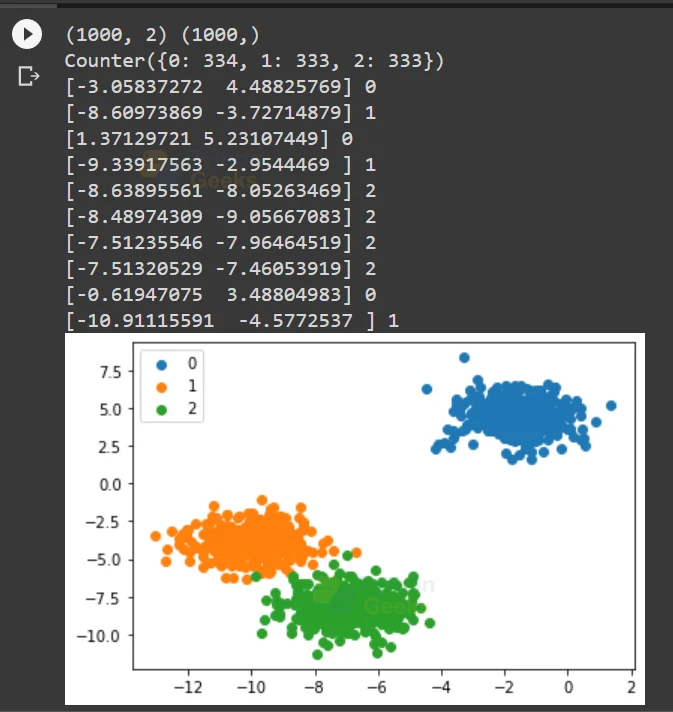
# PythonGeeks example of multi-class classification task
from numpy import where
from collections import Counter
from sklearn.datasets import make_blobs
from matplotlib import pyplot
# define dataset
X, y = make_blobs(n_samples=1000, centers=3, random_state=1)
# summarize dataset shape
print(X.shape, y.shape)
# summarize observations by class label
counter = Counter(y)
print(counter)
# summarize first few examples
for i in range(10):
  print(X[i], y[i])
# we need to plot the dataset and color the by class label
for label, _ in counter.items():
  row_ix = where(y == label)[0]
  pyplot.scatter(X[row_ix, 0], X[row_ix, 1], label=str(label))
pyplot.legend()
pyplot.show()

 

The output of the following multiclass classification code will be

4. Imbalanced Classification

Imbalanced Classification refers to classification tasks where the number of examples in every class is unequally distributed within the dataset.

Typically, imbalanced classification tasks are types of binary classification tasks where the majority of examples in the training dataset have their place in the normal class and the rest of the minority of examples belong to the abnormal class.

Examples of imbalanced classification include:

• Fraud detection.
• Outlier detection.
• Medical diagnostic tests.

We model these problems as binary classification tasks, although they may require specialized techniques.

The code for Imbalanced Classification will be

# PythonGeeks example of an imbalanced binary classification task
from numpy import where
from collections import Counter
from sklearn.datasets import make_classification
from matplotlib import pyplot
# define dataset
X, y = make_classificaation(n_samples=1000, n_features=3, n_informative=3, n_redundant=0, n_classes=2, n_clusters_per_class=1, weights=[0.99,0.01], random_state=1)
# summarize dataset shape
print(X.shape, y.shape)
# summarize observations by class label
counter = Counter(y)
print(counter)
# summarize first few examples
for i in range(10):
  print(X[i], y[i])
# we need to plot the dataset and color the by class label
for label, _ in counter.items():
  row_ix = where(y == label)[0]
  pyplot.scatter(X[row_ix, 0], X[row_ix, 1], label=str(label))
pyplot.legend()
pyplot.show()

The output of the imbalanced classification code will be

Conclusion

With this, we have reached the end of this article that talked about the classification techniques of Machine Learning. We discovered different types of classification predictive modeling in machine learning along with their codes and outputs. Specifically, we learned about Classification predictive modeling which involves assigning a class label to input examples. Hope that this article from PythonGeeks was able to clear your understanding of the concept of Classification in Machine Learning.