Audio Analysis using Deep Learning

You must have come across numerous articles, literature surveys, and other writings that talk about the wonders of Deep Learning in the fields of Natural Language Processing (NLP), Computer Vision, Handling Sequential Data, and various other applications. In this article from PythonGeeks, we will discuss the astonishing field of audio analysis using Deep Learning. This will give you a brief introduction to Automatic Speech Recognition (ASR), digital signal processing, music classification, tagging, and generation. Some of the major Personal Assistants that are popular today like Google Home, Alexa, and Siri make use of the information they extract from audio signals to get our work done in a jiffy.

In this article, we will explore the field of Audio Analysis in a rather comprehensive and easy-to-understand manner. We will cover the introduction about what exactly one means by Audio Analysis, what are the types of audio formats that we deal with, how we can handle data in the form of audio, and the terminologies related to it. Furthermore, we will try to get a brief idea about the processing of the audio signals and the fields of application for audio analysis. So, let’s jump right to the introduction section.

Introduction to Audio Analysis using Deep Learning

As we have studied many times, Machine Learning aims to help Machines gain human-like thinking abilities. We have seen how Machines use neural networks to process inputs related to images, sequential data, and other datasets. However, the human brain isn’t just capable of handling visionary signals, it tends to process audio signals as well.

Right from our communication needs to animals using sound interferences to analyze threats, we surround ourselves with audio signals at any given point. Like visionary inputs, the brain takes the audio signals from the surroundings, processes them, and provides the output stimuli accordingly. Similar to this, developers worldwide are training Machine Learning models to process the audio signals as well. The basis for these audio processing models lies in the foundations of the various audio formats.

We can think of audio format as the quality of the audio data we feed to the models. Based on their applications, we classify the audio formats into three broad parts:

• Uncompressed Format
• Lossy Compressed Format
• Lossless Compress Format

1. Uncompressed Format

The Uncompressed Format has various types of audios related to it. Some of the examples of Uncompressed Audio Formats are:

PCM- PCM is the acronym for Pulse-Code Modulation. The aim of this is to represent raw audio signals in the form of digital signals. This is one of the most common audio formats that finds its applications in CDs and DVDs.

WAV- WAV is the acronym for Waveform Audio File Format. Developed by Microsoft and IBM, it acts as a Windows container for audio formats. Most of the WAV files store uncompressed audio files in the form of PCM.

AIFF- AIFF is the acronym for Audio Interchange File Format. Like WAV, AIFF files also store various kinds of audio and are compatible with both Windows and Mac OS.

2. Lossy Compression Format

Lossy Compressed Format is a form of compression that experiences data loss during compression. Examples of these audio formats are:

MP3- MP3 is one of the widely used audio formats over the globe. It stands for MPEG-1 Audio Layer-3. The main focus of this audio format is to eliminate the unwanted sounds of the background which go unnoticed by the human ears.

WMA- WMA is the acronym for Windows Media Audio, which was designed to remove the drawbacks of MP3. In comparison to MP3, WMA has a better audio quality index.

3. Lossless Compress Format

Lossless Compression is the method of reducing file size without any loss of data. The examples of Lossless Compression are:

FLAC- Free Lossless Audio Codec is a method that can compress an audio file by 50% without suffering any data loss.

ALAC- Apple Lossless Audio Codec is another invention by Apple for audio compression with minimum possible data loss.

Now that we know some details about the audio formats, let us look at the data handling mechanism in audio analysis.

Python Audio Libraries

Python provides us with some great libraries for audio processing like Librosa and PyAudio. There also exist built-in modules for some preliminary audio functionalities.

1. Librosa

Librosa is a Python module that helps us to analyze audio signals in general and is geared more towards music. It consists of the nuts and bolts to build a MIR(Music information retrieval) system.

2.IPython.display.Audio

This Python library allows you to play audio files directly through the jupyter notebooks.

Data Handling in Audio Domain

As we have seen in the earlier sections, audio files in their raw form, have unstructured data format. In order to efficiently process this audio data, we have to perform some preprocessing steps that are necessary for the processing of the audio input.

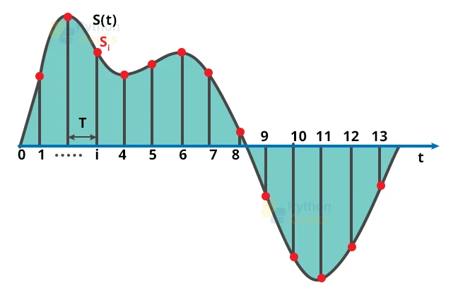
As a beginning step, we have to convert loaded data into a format that is easily read by the machine-readable format. For doing so, we simply observe the values of the input after a specified time interval. As an example, we can extract the data from a 2-second audio file for every half second. This process is commonly referred to as the sampling of audio data. The rate that we decide to extract the data from the audio file is the sampling rate.

The necessary conditions for the sampling of audio files are, we need to consider more data points to represent the sampling data, and secondly, we need to have a high sampling rate. By doing so, we will require a minimum computational power for the representation of audio data in the frequency domain.

As an example, for a better understanding of the sampling problem, consider the image below. Here, we need to split a single audio signal into three pure signals for the convenient representation of the signal as three unique values in the frequency domain. There are other ways as well for the representation of audio signals other than this method like MFC. This representation helps the model in the extraction of distinct features from the audio file. The trained models then process these extracted features and perform the necessary tasks they are required for audio processing.

Let us now go through the basic terms that are related to the audio processing models.

Terminologies for Audio Processing

Sampling: In the processing of signals, the reduction of a continuous signal into a series of discrete values is known as sampling. The number of samples that we extract for the fixed interval of time is the sampling frequency or sampling rate. Higher sampling frequency ensures lesser data loss but requires higher computational expense.

Amplitude: Amplitude is the most common term associated with audio signals. It is the measure of the change in the magnitude of the frequency of the audio signals over a period of time.

Fourier Transform: The main aim of the Fourier Transform is to decompose the function of time into its constituent frequencies. For audio signals, Fourier Transform decomposes the volumes and frequencies associated with the audio signal and displays the amplitude and frequency of the underlying function.

Periodogram: The estimation of the spectral density of a signal in signal processing is known as a periodogram. The output of the Fourier Transform of the audio signal can be thought of as a periodogram.

Spectral Density: To understand the spectral density, we first need to understand the power spectrum. The way to describe the distribution of power into discrete frequency components of any time series as a composition of their signal is the power spectrum. The spectrum of the signal is the statistical average of its frequency content. Similarly, the description of the frequency content of a digital signal is known as Spectral Density.

Spectrum: As we have seen earlier, we can add signals of different frequencies together to create composite signals, representing any sound that occurs in the real world. In simple words, any signal consists of many distinct frequencies and we can express them as the sum of those frequencies. The Spectrum is the set of such frequencies that are we combine together to produce a signal. As an example, consider the picture shows the spectrum of a piece of music. The Spectrum will plot all of the frequencies that are present in the signal in addition to the strength or amplitude of each frequency.

Spectrogram: A spectrogram helps us to visually represent the signal strength or the “loudness” of a signal over time at various frequencies that exist in a particular waveform. Not only can you observe whether there is more or less energy at, for example, 2 Hz vs 10 Hz, but you can even observe how energy levels vary over time.

Generation of Spectrogram: We can generate spectrograms using Fourier Transforms in order to segregate the signals into their constituent frequencies.

Now that you are familiar with the terminologies related to audio processing, let us take a look at the audio processing mechanism of digital signals.

Time-domain vs Frequency domain

The waveforms that we have seen earlier showing Amplitude against Time are one of the ways to represent a sound signal. Since the x-axis represents the range of time values of the signal, we will observe the signal in the Time Domain. The Spectrum is an alternative for the representation of the same signal. It represents the Amplitude against Frequency, and since the x-axis represents the range of frequency values of the signal, at an instance in time, we are observing the signal in the Frequency Domain.

Feature Extraction from Audio Signals

Every audio signal contains many features. However, you must extract the characteristics that are relevant to the problem we are concerned with. The process of extracting features to utilize them for analysis is called feature extraction. Let us look at a few of the features in brief.

The spectral features (frequency-based features), which we obtain by converting the time-based signal into the frequency domain using the Fourier Transform, like fundamental frequency, frequency components, spectral centroid, spectral flux, spectral density, spectral roll-off, and so on.

Music Genre Classification

The dataset that was used for the well-known paper in genre classification “Musical genre classification of audio signals” by G. Tzanetakis and P. Cook in IEEE Transactions on Audio and Speech Processing 2002.

The dataset that was used here consists of 1000 audio tracks each 30 seconds long. It contains 10 genres, each represented by 100 tracks. The tracks were all 22050 Hz monophonic 16-bit audio files that were in .wav format.

The dataset for this problem consisted of 10 distinct genres for the classification of the audio files, namely, Blues, Classics, Country, Disco, Metal, Jazz, HipHop, Rock, Reage, and Rock.

The roadmap for the following dataset was:

In order to implement the genre classification, first of all, we need to convert the audio files (10 of each genre) into PNG format images(spectrograms). From these visual representations from the spectrograms, we have to extract meaningful features, like MFCCs, Spectral Centroid, Zero Crossing Rate, Chroma Frequencies, and Spectral Roll-off.

Once we extract these meaningful features, we can append them into a CSV file so that we can use ANN for the classification of the music genres.

The general algorithm for this classification involves the following steps:

1. We first need to extract and load our data to Google Drive in order to mount it on the Colab notebook.

2. We then need to import all the necessary libraries for the extraction of the data

3. For a visual representation, we need to convert these audio files into PNG format images. In simple words, we need to extract the Spectrogram for each audio set. We perform this step in order to make it easy for us to extract the features of the audio.

4. We then need to create a header for our CSV file.

5. This step is the most crucial step of the algorithm. We now have to extract the features like MFCC, Spectral Centroid, Zero Crossing Rate, and Chroma Frequencies.

6. In this step, we load the CSV data, label encoding, and feature scaling. We tend to split the data for training the data set.

7. The next step involves building the ANN model.

8. As the final step, we fit in the model.

Processing Audio: Digital Signal Processing Techniques

For processing any kind of dataset, we need to extract the features of the dataset and engineer the feature processing on the particular dataset. In order to perform these operations on the audio analysis, we need to engineer the components of the audio signals that will help us in finding distinguishing features of the signals.

The most common tool for the extraction of information from audio signals is MFCCs. Despite having one-liner python codes to compute MFCCs of the audio signals, the actual math related to the computational process is quite complex. The underlying steps for the calculation of MFCCs are:

1. Slicing of the signal into shorter frames.
2. Computing the periodogram estimation of the power spectrum for each frame.
3. Applying the mel-filterbank to the power spectra.
4. Taking the discrete cosine transform (DCT) of log filterbank energies.

Now that we know the processing of audio signals, let us dive into the application of the Audio Analysis section.

Applications of Audio Analysis

1. Audio Classification

The classification problem aims to extract useful features from the input audio signal and identify the class to which the audio belongs. It is a fundamental problem in the audio analysis field. Major tech giants make use of audio classification for a variety of different uses such as genre classification, instrument recognition, and the identifications of the artists.

2. Audio Fingerprinting

The focus of this audio analysis problem is to establish a digital “summary” of the audio. We perform this in order to uncover the main audio file from the sample audio input. One of the most popular examples of audio fingerprinting is Shazam. It is used to search for the song on the basis of the sample audio that we feed to the input layer. The major drawback of the system is the lack of clarity of the main audio due to background noises.

3. Audio Segmentation

The actual meaning of segmentation is to bifurcate the original piece of information into smaller parts on the basis of a particular set of characteristics. For any audio processing unit, segmentation acts as an important preprocessing step. The main usage of the segmentation of the audio signal is, we can segment a lengthy noisy audio file into a homogenous shorter version.

4. Audio Source Separation

When the audio signals contain a mixture of signals, audio source separation is used to separate the various source signals from each other. One of the most used applications of this technique is the extraction of lyrics from the audio file for karaoke.

5. Music Genre Classification and Tagging

With the increase in popularity of music streaming services, another explicit application that most of us are familiar with is to identify and categorize music on the basis of audio. We first analyze the content of the music is to figure out the genre to which the audio belongs. This comprises a multi-label classification problem as a given piece of music may tend to fall under more than one genre.

6. Music Generation and Music Transcription

As we have seen earlier, a lot of news these days talk about deep learning being used to programmatically generate extremely authentic-looking pictures of faces and other scenes. Apart from these, it is able to write grammatically correct and intelligent letters or news articles. In a similar sense, we are now able to fabricate synthetic music that can precisely match a particular genre, instrument, or even a given composer’s style.

Other Applications

Apart from the above applications, audio analysis is useful for a variety of other tasks. Audio analysis is useful for indexing music collections according to their audio features. It acts as a wonderful tool for music recommendation systems for radio stations. It is also useful for speech processing and synthesis.

Conclusion

Thus, we came across one more fascinating application of Audio Analysis using deep learning. Now, you will be able to identify the audio analysis problems, it’s working, and the different terminologies related to the audio processing. We also saw some of the major applications of Audio Analysis. Hope this PythonGeeks article was useful for your understanding of Audio Analysis.