Data Preprocessing in Machine Learning

Data preprocessing is the procedure for making raw data into a suitable form, so it is ready for machine learning. Data is gathered from different sources and cleaned up to be prepared for machine learning. It may contain noises and missing data or may not be in a suitable form.

However, it must be in an organised format to apply machine learning algorithms to get correct predictions. Let’s learn more about Data Preprocessing in Machine Learning.

Why Do We Need Data Preprocessing?

Real-time data contains lots of missing values and distortions. For machine learning to give correct outputs, it must go through a series of steps so the data is organised and is in a standard format. Cleaned data increases the accuracy and efficiency of the learning model.

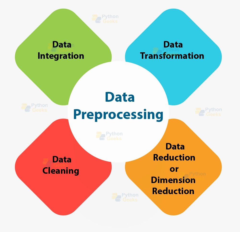
Different Techniques of Data Preprocessing

1. Rescale Data

If our datasets contain data with different scales, rescaling can make the job of the machine learning algorithms easier. This method is primarily helpful in gradient descent.

You can use the MinMaxScaler class for rescaling.

2. Binarize Data (Convert Data into Binary Format)

We assign a threshold, and all values above the threshold are considered 1. Then, all values below the threshold are considered 0. It is useful when you want to convert probabilities into crisp values.

The binarizer class in scikit-learn helps to convert new binary attributes.

3. Standardise Data

It is the method of transforming attributes with a gaussian distribution and ranging mean and standard deviation to gaussian distribution with mean value 0 and standard deviation as 1. We will look into the method further in this article.

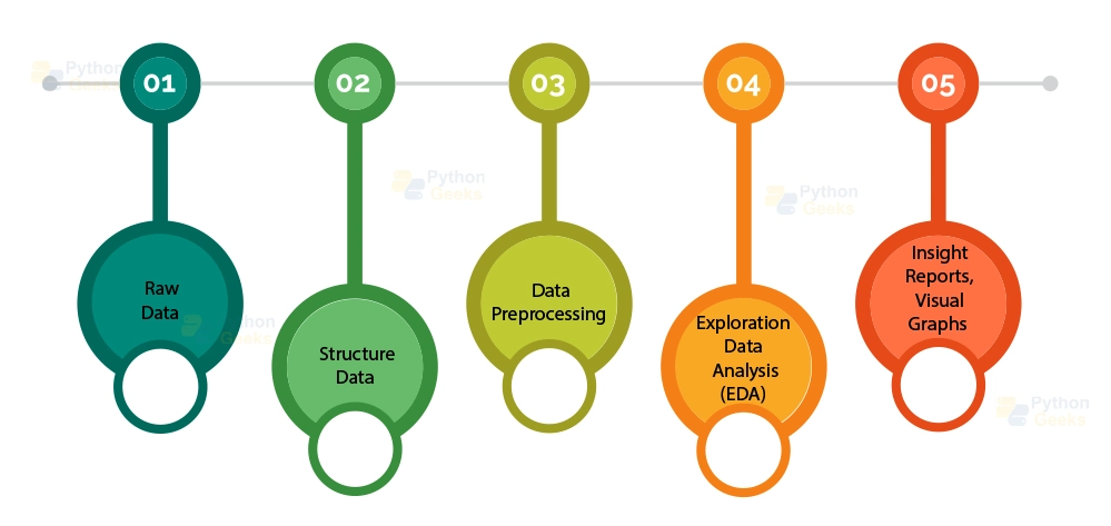
Steps of Data Preprocessing

1. Getting the dataset

Machine learning models work on data. Thus, we require a dataset to build a machine-learning algorithm.

Datasets are in different forms and formats. For example, the dataset for breast cancer detection will be different from the dataset for customer analysis. A dataset is usually in a CSV format. We could also use HTML and XML files.

What is a CSV file?

CSV is the abbreviation of Comma-Separated Values. CSV files present data in tabular format. Therefore, it is helpful in storing data for machine learning.

In this article, we will use Anaconda and export the dataset to perform data preprocessing. Use the link to download dataset in CSV format:

2. Importing libraries

The next step is to import libraries. These libraries are pre-defined in Python, and they perform certain vital functions. The following are the three most important libraries used in machine learning.

a. Numpy

The numpy is a Python library that helps define dimensional arrays and many other mathematical operations in Python. It also performs many other mathematical and scientific calculations.
Import numpy as np.

b. Matplotlib

This library is used for creating graphs and plotting 2D libraries in Python. The sublibrary is known as pyplot, which helps to plot charts and other graphical representations. It helps us understand our data better.

c. Pandas

Pandas is an extremely popular library in Python. With the help of this library, we can import and manage datasets in Python. Moreover, it is an open-source library. We can use the following command to import the library:

Import pandas as pd

3. Importing the Datasets

Once we import the libraries, the first step is to import the datasets. Only then can we manipulate the data present to work on our algorithms. We must ensure the current directory is the working directory. The dataset is simple and easy to import.

df= pd.read_csv(r'C:\Users\qures\Downloads\sample.csv')
print(df)

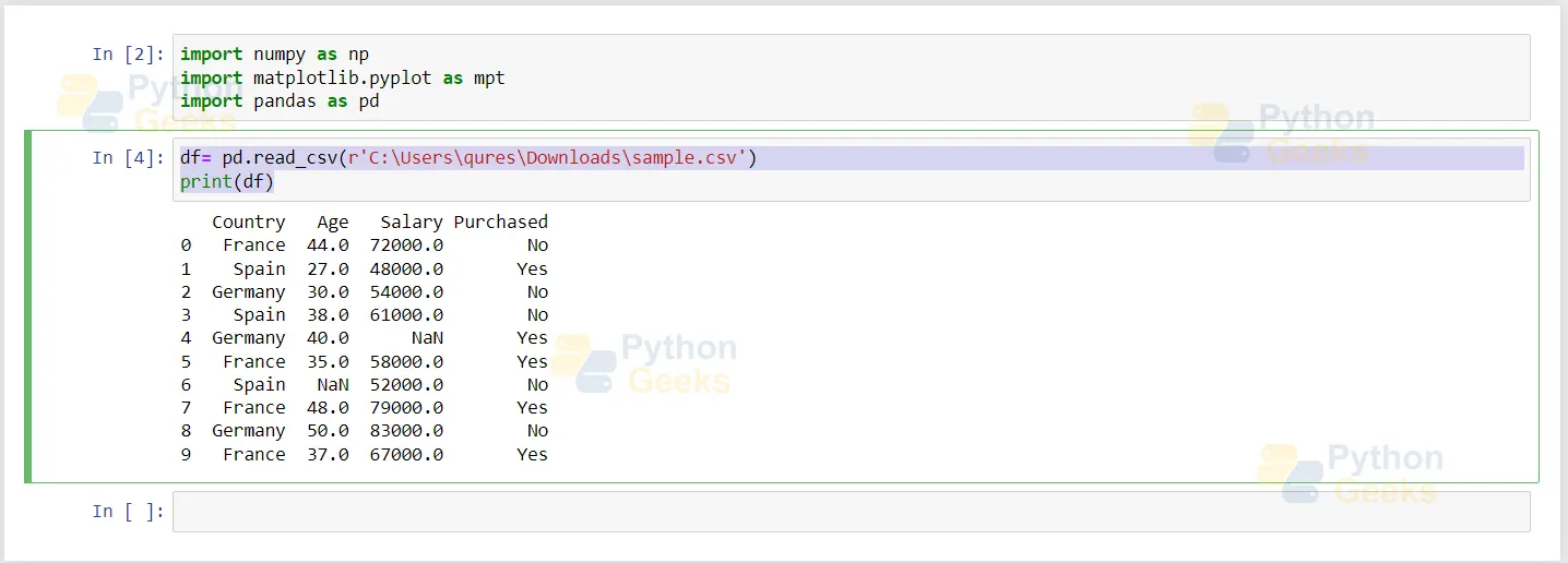
If we look at the data carefully, we will notice incomplete values and inconsistencies. It means that the dataset is not suitable for machine learning as this has different unnecessary values. Therefore, we need to perform data preprocessing.

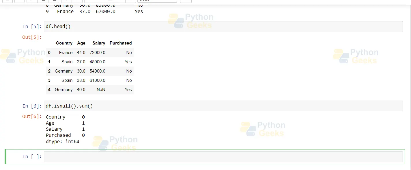
df.head() returns the first five values of the dataset

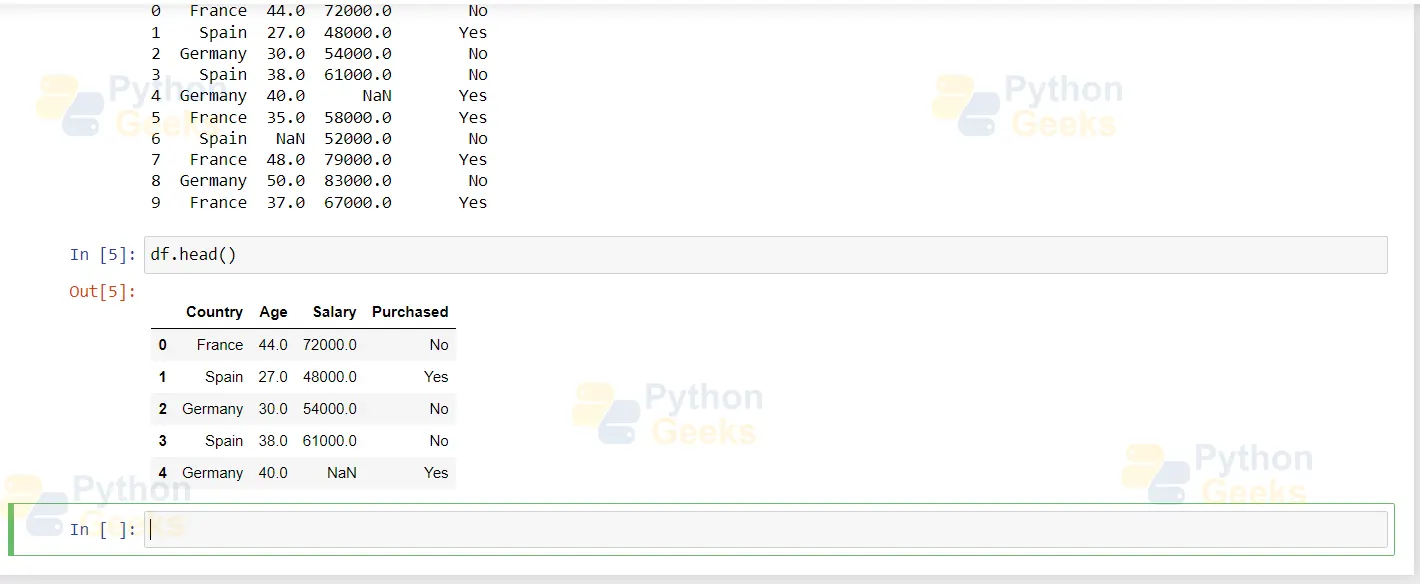
All the changes to the data can be made by looking at these dataset values. However, machine learning algorithms cannot understand string data such as France, Germany and Spain given in a dataset. So we feed this kind of data in the form of numbers.

If values are not available, we consider them as null values. To check for null values, type the following commands:

df.isnull().sum()

4. Splitting the Data into x and y Values

Y is dependent on x. It learns the correlation existing between the data by learning from the dataset.

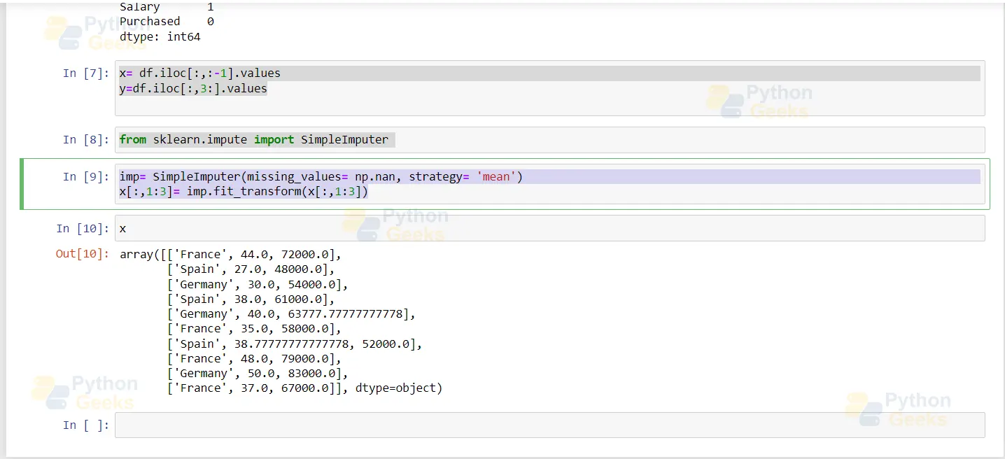
x= df.iloc[:,:-1].values
y=df.iloc[:,3:].values

Simpleimputer is a package in sklearn that fills in the missing values. Missing values can be filled with the help of strategies such as filling them with the mean median or mode of the particular column of the dataset. Another way is to fill in the most common value or delete the entire row.

from sklearn.impute import SimpleImputer

Here we are using the mean strategy to fill our input values.

imp= SimpleImputer(missing_values= np.nan, strategy= 'mean')
x[:,1:3]= imp.fit_transform(x[:,1:3])

5. Handling Categorical Values

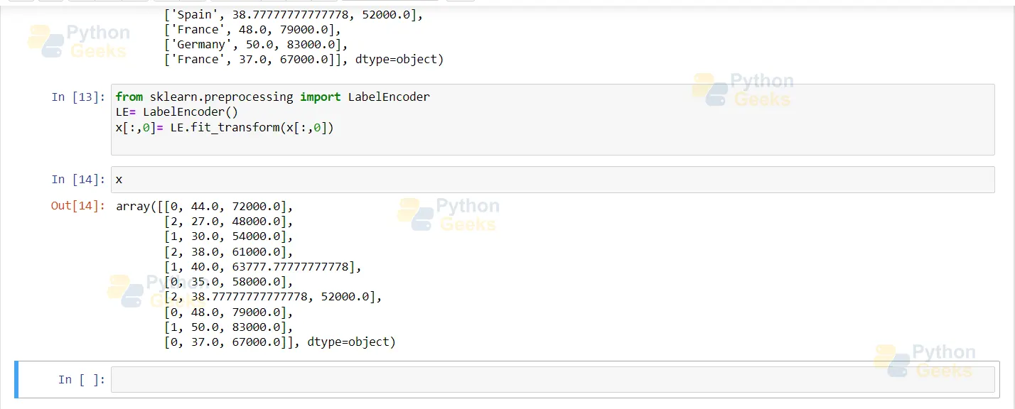
In our dataset, France, Germany, and Spain are categorical values that must be changed. So we assign numbers to these values.

France- 0
Germany- 1
Spain- 2

Then, paste these values into the original data.

Labelencoder is the method to apply this directly in Python. It is used for encoding labels.

Then, paste these values into the original data.

Labelencoder is the method to apply this directly in Python. It is used for encoding labels.

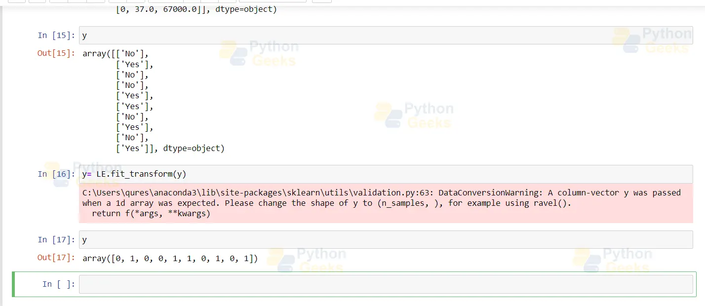
As we can see below, our data is split into categorical values, and it must undergo transformation.

y 
y= LE.fit_transform(y)
y 

Handling Null Values

In real-world datasets, there are always null values. These null values cause interruptions, and no model can handle the null values. So we need to remove these before applying them to any machine learning algorithm.

Firstly, we must confirm if our dataset contains NULL or NaN values. It is done with the in-built function isnull().

We can drop the rows and columns containing these null values to remove these null values. But it is not the best way to tackle the problem. Sometimes dropping entire rows and columns from the dataset eliminates some valuable data. So one way to handle these issues is Imputation.

Imputation

It is a method used to substitute the null values with some other values. It is done with the help of the SimpleImputer class in sklearn.

Standardisation

Standardisation is another method to tackle null values. The mean of these values is null. So the standard deviation sums to 1. Basically, we calculate each data point’s mean and standard deviation, remove the mean, and divide the standard deviation.

OneHotEncoding

We use this method when we have several categorical values of more than 3. Imagine we have a dataset with 3 categorical values. The issue arises when we take the average of the values. So it computes the average of France and Germany to Spain.

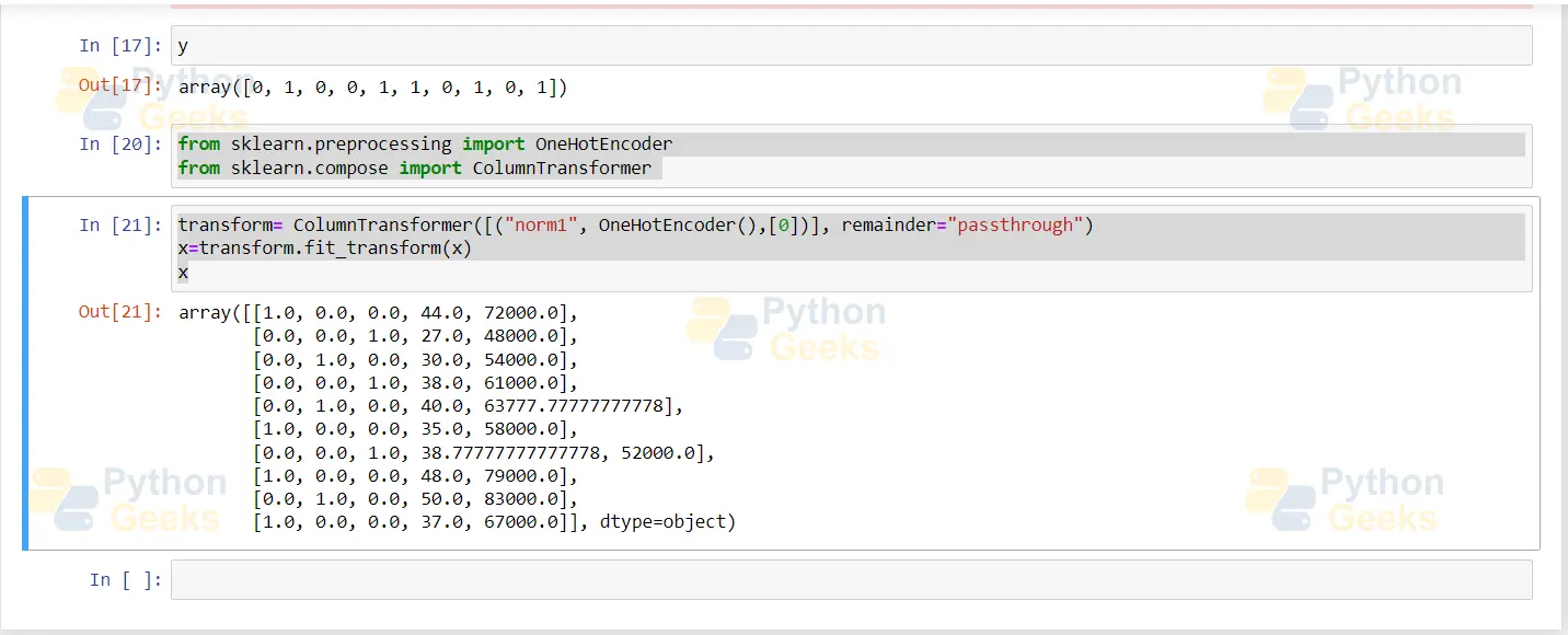
Given below is the code for performing OneHotEncoding:

from sklearn.preprocessing import OneHotEncoder 
from sklearn.compose import ColumnTransformer 
transform= ColumnTransformer([("norm1", OneHotEncoder(),[0])], remainder="passthrough")
x=transform.fit_transform(x)
X

And this is the code screenshot

Multicollinearity and Its Impact

Strongly independent features give rise to multicollinearity. So we use a weight vector to calculate feature importance, which is impossible to calculate if we have multicollinearity in our dataset.

How to Avoid Multicollinearity?

If we want to avoid multicollinearity, we can use drop_first = True. It does not lead to any information loss. Only the strong correlation between columns is broken.

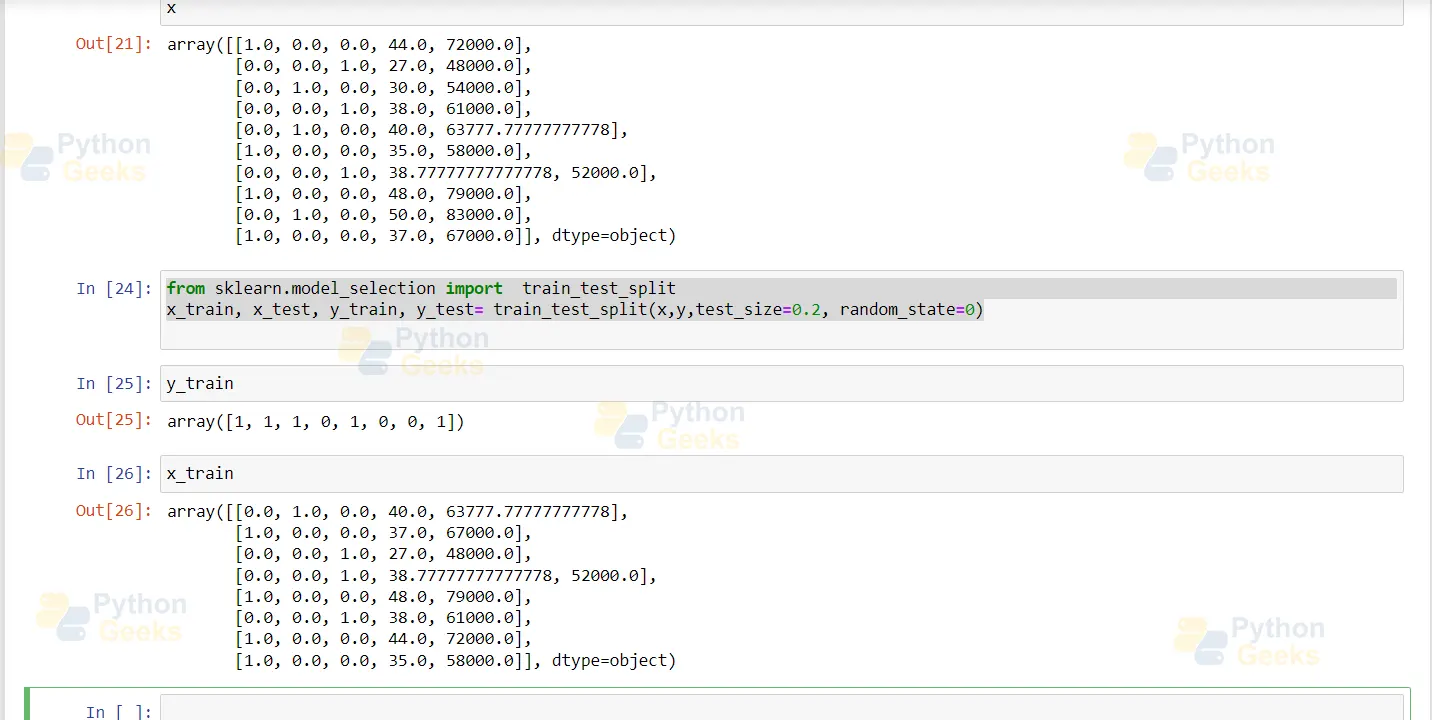
Split the data into training and testing

70% of the data is used for training the model, and we will use the rest for testing. Below is the code:

from sklearn.model_selection import train_test_split
x_train, x_test, y_train, y_test= train_test_split(x,y,test_size=0.2, random_state=0)

Apply standard scaler

Procedure for applying standard scalar:

y=(x-mean)/standard_deviation
mean= sum(x)/count(x)
standrd_deviation= sqrt((x-mean)^2)/count(x))

from sklearn.preprocessing import StandardScaler
sc= StandardScaler()
x_train[:,3:5]= sc.fit_transform(x_train[:,3:5])
x_train

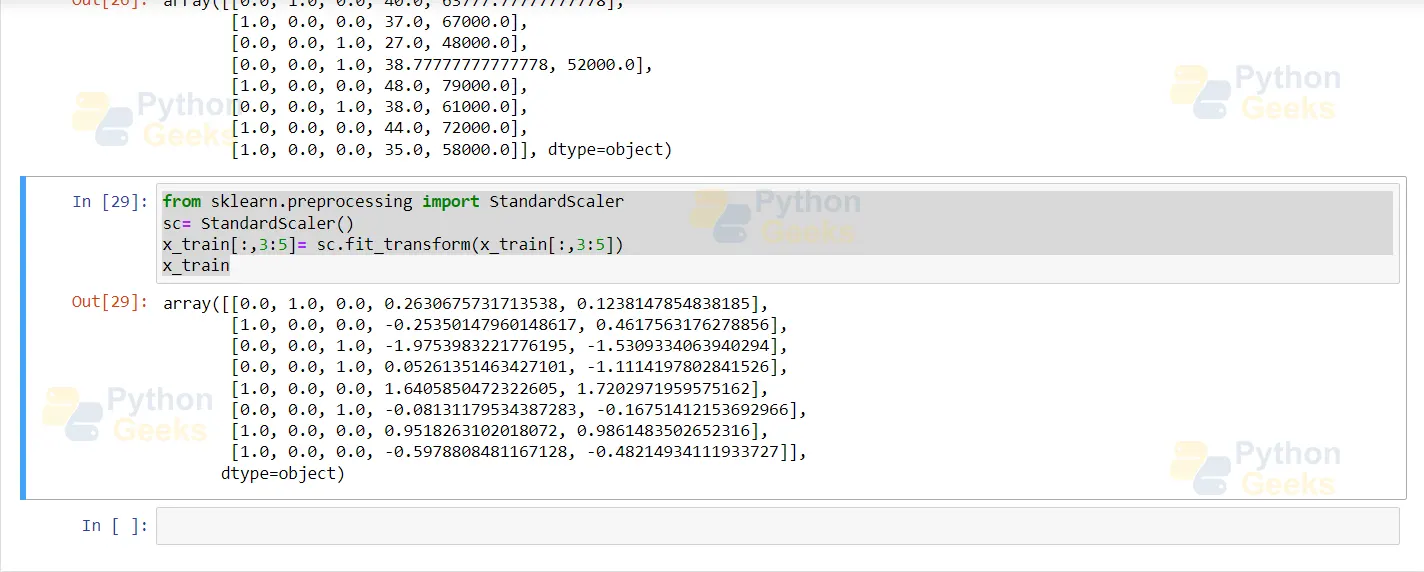
The standard scaler fits our data in the range of 0 and 1. Therefore, the data in the above screenshot is perfectly feedable to our machine learning model for the application of any algorithm, such as linear regression and classification.

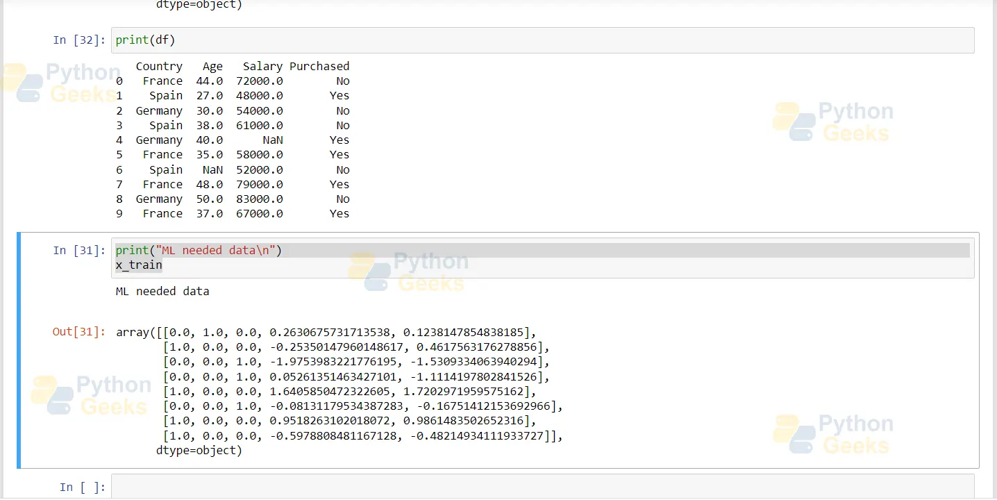
Finally, let us have a look at the original dataset at the start of the tutorial:

print(df)
print("ML needed data\n")
x_train

We can see the difference in the dataset now; this data form is ready to be applied to any machine learning algorithm.

Conclusion

In this article we have learnt the steps of data preprocessing in machine learning. It is one of the most time consuming and important steps in ML. We looked at various ways to process the data such as handling null values, one hot encoding, standardisation and so on.