Dilation and Erosion in OpenCV

In this article, we’ll thoroughly understand the dilation and erosion morphological operations in OpenCV. But before we start, let us see what are these operations.

Morphological operations in OpenCV

Erosion and dilation come under morphological operations. Morphological operations are a set of operations for image processing based on the shape of the image. Morphological operations are performed on binary images and require two inputs, the source image and a structuring element or kernel.

The structuring element is determined on the basis of the input image given. The morphological operations aim to remove noise and settle imperfections, to make the image sharper and clearer.

In the morphological operations, the value of each pixel in the output image is computed on the basis of the comparison of the value of the pixel in the input image with the pixels in its neighborhood.

Pixels are added to the boundaries of the objects in an image using dilation, whereas pixels are removed or essentially, eroded from the boundaries of the objects in an image using erosion. The number of pixels that are to be added or removed from the boundaries of the objects depend on the structuring element developed on the basis of the input image.

In the morphological dilation and erosion operations, the state for the pixels is determined by applying a rule to the corresponding pixel and the pixels in its neighbourhood in the input image. The rule which is used to process the pixels of the image, defines whether the operation to be performed is dilation or erosion.

Dilation in OpenCV

It is a method of adding pixels to the boundaries of objects in an image. Dilation of the image is done by convolution of the image with a kernel of specified shape.

The kernel has an anchor point which is by default positioned at the center of the kernel. The kernel is overlapped with the image and computes the maximum value for the pixel. After determining the maximum value of the pixel, it is replaced with the image pixel value at the anchor point at the center. This procedure is repeated. After dilation, the areas around the boundaries of the objects grow in size and the size of the image also increases.

Working of dilation

1. In dilation, the image is convolved with a kernel of odd size.
2. The kernel travels through the image and searches for a similar pattern.
3. If at least one pixel under the kernel is 1, then the central pixel is set to 1, otherwise the pixel is set to 0.
4. After traversing through the image, the white region in the image increases.

Mathematically, dilation operation is:

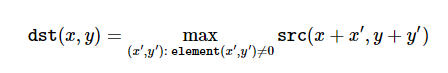
In dilation, the structuring element i.e. the kernel travels through the image and searches for a pattern resembling its structure. Wherever the image pattern and structuring element pattern have one matched pixel, the output pixel is written a 1 and the output pixel is written as 0 if they don’t.

Syntax

cv2.dilate(src, kernel, anchor, iterations, borderType, borderValue)

Parameters

• src: Source image or input image over which we’ll be performing dilation
• kernel: Required parameter with which the image is convolved. It is also referred to as the structuring element and the shape and size of the
• kernel is decided on the basis of the input image.
• dst: Output image of the same size and type as the input image.
• anchor: It is the position of the anchor within the element. By default, the position is at the center of the element.
• iteration: Specifies number of times dilation is applied
• borderType: Type of border. It is a pixel extrapolation method.
• borderValue: It is the border value for a constant border.

Implementation of dilation in opencv

# Importing OpenCV
import cv2

# Importing numpy
import numpy as np

# Reading image
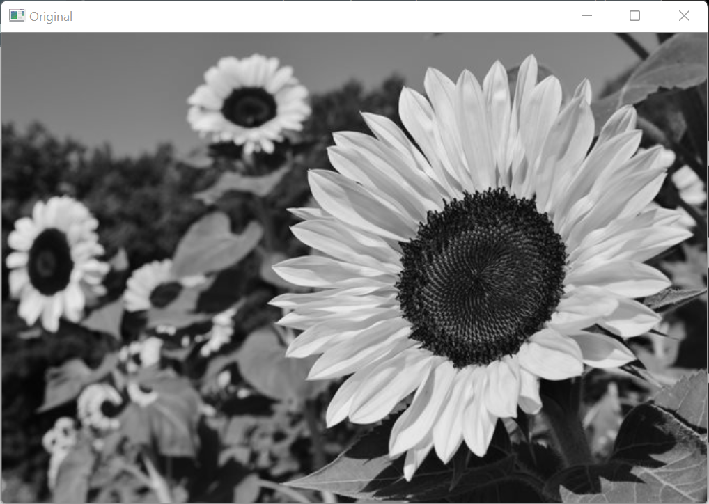
img = cv2.imread(r"C:\Users\tushi\Downloads\PythonGeeks\flower.jpg",0)

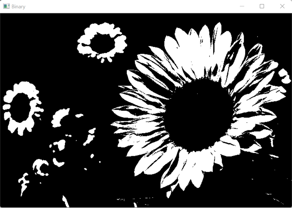
# Converting grayscale image to binary using thresholding
ret, img_binary = cv2.threshold(img, 175, 255, cv2.THRESH_BINARY)

# Displaying the original image and binary image
cv2.imshow('Original',img)
cv2.imshow('Binary', img_binary)
cv2.waitKey(0)
cv2.destroyAllWindows()

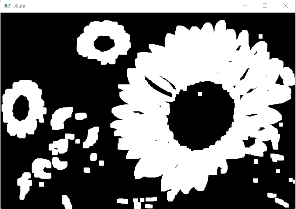
# Defining kernel
kernel = np.ones((5,5),dtype=np.uint8)

# Applying dilation operation
img_dilate = cv2.dilate(img_binary, kernel, iterations=2)

# Displaying the dilated image
cv2.imshow('Dilate', img_dilate)
cv2.waitKey(0)
cv2.destroyAllWindows()

Uses of Dilation

1. Morphological dilation makes objects sharper and more visible.

2. It helps in filling any small holes in the image.

3. For noise removal, erosion is followed by dilation to enhance the image after the removal of the noise.

Erosion in OpenCV

Erosion is the method for eroding the boundaries of foreground objects. In this operation, the pixels near the boundaries of the objects will be discarded depending upon the size of the kernel. The thickness or size of the foreground object or the white region in the image decreases due to erosion.

The erosion operation computes the local minimum over the area of the kernel. The image is overlapped with the kernel and the pixel value at the anchor point positioned at the center of the kernel is replaced with the minimum value calculated.

In Erosion, the structuring element i.e. the kernel travels through the image and searches for a pattern resembling its structure. Wherever the image pattern and structuring element pattern have one matched pixel, the output pixel is written as 1 and the output pixel is written as 0 if they don’t.

Working of erosion

1. In erosion, the image is convolved with an odd size kernel.
2. The kernel travels through the image and searches for a similar pattern
3 If all pixels under the kernel are 1, then the central pixel is set to 1, otherwise the pixel is set to 0.
4. Pixels near the boundary of the objects in the image are set to 0 depending on the size of the structuring element.
5. After traversing through the image, the white region in the image decreases.

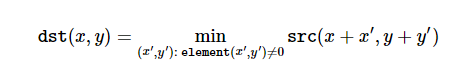
Mathematically, the shape of the pixel neighborhood over which the minimum value is computed is:

Syntax

cv2.erode(src, kernel, dst, anchor, iterations, borderType, borderValue)

Parameters of OpenCV Erosion

• src: It is the input image or the source image
• dst: Output image of the same size and type as the source image
• kernel: It is the structuring element used for erosion.
• anchor: It is the position of the anchor within the element. By default, the position is at the center of the element.
• iteration: Specifies the number of times erosion is applied.
• borderType: Type of border. It is a pixel extrapolation method.
• borderValue: It is the border value for a constant border.

OpenCV Erosion Implementation

# Importing OpenCV
import cv2

# Importing numpy
import numpy as np

# Reading image
img = cv2.imread(r"C:\Users\tushi\Downloads\PythonGeeks\flower.jpg",0)

# Converting grayscale image to binary using thresholding
ret, img_binary = cv2.threshold(img, 175, 255, cv2.THRESH_BINARY)

# Displaying the original image and binary image
cv2.imshow('Original',img)
cv2.imshow('Binary', img_binary)
cv2.waitKey(0)
cv2.destroyAllWindows()

# Defining kernel
kernel = np.ones((5,5),dtype=np.uint8)

# Applying erosion operation
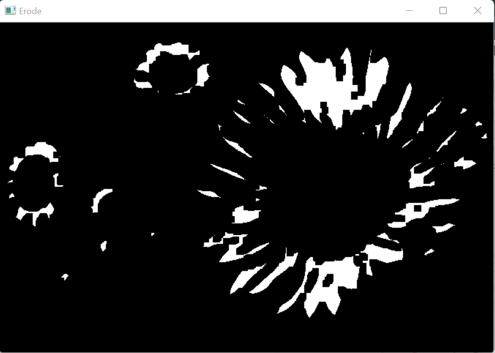
img_erode = cv2.erode(img_binary, kernel, iterations=2)

# Displaying the eroded image
cv2.imshow('Erode', img_erode)
cv2.waitKey(0)
cv2.destroyAllWindows()

Uses of erosion

1. It enlarges foreground holes.

2. It is useful for shrinking foreground objects

3. It removes small noises from the image.

4. It detaches two connected objects.

Log Transformation in OpenCV

Logarithmic Transformation in OpenCV is used for image transformation on the basis of the intensity values of the pixels. The value for each pixel in the image is replaced by their logarithmic values. The Log transformation is used to enhance the contrast of the image.

Syntax

cv2.intenstity_transform.logTransform(input, output)

Parameters

• input: Input image used for transformation
• output: Output image of the same size and type as the input image.

Implementation

# Importing OpenCV
import cv2
 
# Importing numpy
import numpy as np
 
# Importing matplotlib.pyplot
import matplotlib.pyplot as plt
 
# Reading an image 
img = cv2.imread(r"C:\Users\tushi\Downloads\PythonGeeks\flower.jpg")
img = cv2.cvtColor(img, cv2.COLOR_BGR2RGB)
 
# Setting the grid size
plt.figure(figsize=(10,10))
 
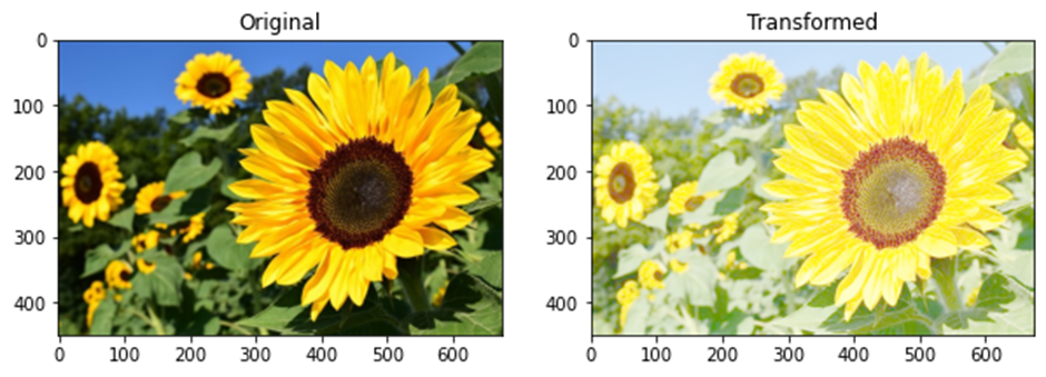
# Plotting the original image
plt.subplot(121)
plt.title('Original')
plt.imshow(img)
 
# Applying Logarithmic transformation
cv2.intensity_transform.logTransform(img, img)
 
# Plotting the transformed image
plt.subplot(122)
plt.title('Transformed')
plt.imshow(img)

Piecewise Linear Transformation in OpenCV

The piecewise Linear transformations are not entirely linear in nature. The function is linear between certain x-intervals. Contrast stretching is the most commonly used piecewise Linear transformation.

Contrast stretching is used to increase the range of intensity levels in the image. The function increases monotonically.

Contrast can be expressed by the given equation:

Contrast = (Maximum Intensity – Minimum Intensity)(Maximum Intensity + Minimum Intensity)

Syntax

cv2.intensity_transform.contrastStretching(input, output, r1, s1, r2, s2)

Parameters

• input: Input image used for transformation
• output: Output image of the same size and type as the input image.
• r1: The x coordinate for the first point in the function (r1, s1)
• s1: The y coordinate for the first point in the function (r1, s1)
• r2: The x coordinate for the second point in the function (r2, s2)
• s2: The y coordinate for the second point in the function (r2, s2)

Implementation

# Importing OpenCV
import cv2
 
# Importing numpy
import numpy as np
 
# Importing matplotlib.pyplot
import matplotlib.pyplot as plt
 
# Reading an image 
img = cv2.imread(r"C:\Users\tushi\Downloads\PythonGeeks\flower.jpg")
img = cv2.cvtColor(img, cv2.COLOR_BGR2RGB)
 
# Setting the grid size
plt.figure(figsize=(20,20))
 
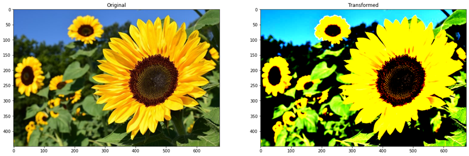
# Plotting the original image
plt.subplot(121)
plt.title('Original')
plt.imshow(img)
 
# Applying Contrast stretching transformation
cv2.intensity_transform.contrastStretching(img, img, 70, 0, 140, 255)
 
# Plotting the transformed image
plt.subplot(122)
plt.title('Transformed')
plt.imshow(img)

Denoising images in OpenCV

Denoising an image is the process of removing unwanted signals and information from the image. It is the process of retaining only the useful information of the image. It is used for better analysis of images. Denoising an image is an essential step in image processing.

There are four variants of Denoising technique in OpenCV:

1. cv2.fastNIMeansDenoising()

This function works with a single grayscale image

Syntax

cv2.fastNIMeansDenoising(src, dst, h, templateWindowSize, searchWindowSize)

Parameters

• src: Input image. It should be 8-bit. The image can have up to four channels.
• dst: Output image of the same size and type as the input image
• h: This parameter regulates the strength of the filter. For higher value of h, more noise and details are removed from the image and vice versa.
• templateWindowSize: Size of template patch in pixels. It computes the weights. The size of the template window should be odd.
• searchWindowSize: Size of the search window in pixels. It is used to calculate the weighted average. The size of the search window should be odd.

2. cv2.fastNIMeansDenoisingColored()

This function works with a color image.

Syntax

cv2.fastNIMeansDenoisingColored(src, dst, h, hcolor, templateWindowSize, searchWindowSize)

Parameters

• src: Input image. It should be 8-bit. The image can have up to four channels.
• dst: Output image of the same size and type as the input image
• h: This parameter regulates the strength of the filter. For higher value of h, more noise and details are removed from the image and vice versa.
• hcolor: h parameter for color components
• templateWindowSize: Size of template patch in pixels. It computes the weights. The size of the template window should be odd.
• searchWindowSize: Size of the search window in pixels. It is used to calculate the weighted average. The size of the search window should be odd.

3. cv2.fastNIMeansDenoisingMulti()

This function works with a sequence of images that has been captured in a small time.

Syntax

cv2.fastNIMeansDenoisingMulti(src, imgToDenoiseIndex, dst, temporalWindowSize, h, templateWindowSize, searchWindowSize)

Parameters

• src: Sequence of input images. The images should be 8-bit. The images can have up to four channels.
• imgToDenoiseIndex: The current image to denoise from the image sequence
• temporalWindowSize: It specifies the number of images to be used that surround the target image for denoising.
• dst: Output image of the same size and type as the input image
• h: This parameter regulates the strength of the filter. For higher value of h, more noise and details are removed from the image and vice versa.
• templateWindowSize: Size of template patch in pixels. It computes the weights. The size of the template window should be odd.
• searchWindowSize: Size of the search window in pixels It is used to calculate the weighted average. The size of the search window should be odd.

4. cv2.fastNIMeansDenoisingColoredMulti()

This function works with a sequence of images that has been captured in a small time for colored images.

Syntax

cv2.fastNIMeansDenoisingColoredMulti(src, imgToDenoiseIndex, dst, temporalWindowSize, h, hcolor, templateWindowSize, searchWindowSize)

Parameters

• src: Sequence of input images. The images should be 8-bit. The images can have up to four channels.
• imgToDenoiseIndex: The current image to denoise from the image sequence
• temporalWindowSize: It specifies the number of images to be used that surround the target image for denoising.
• dst: Output image of the same size and type as the input image
• h: This parameter regulates the strength of the filter. For higher value of h, more noise and details are removed from the image and vice versa.
• hcolor: h parameter for color components.
• templateWindowSize: Size of template patch in pixels. It computes the weights. The size of the template window should be odd.
• searchWindowSize: Size of the search window in pixels. It is used to calculate the weighted average. The size of the search window should be odd.

Implementation

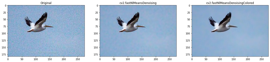
1. cv2.fastNlMeansDenoising() and cv2.fastNlMeansDenoisingColored() function

# Importing OpenCV
import cv2
 
# Importing numpy
import numpy as np
 
# Importing matplotlib.pyplot
import matplotlib.pyplot as plt
 
# Reading an image 
img = cv2.imread(r"C:\Users\tushi\Downloads\PythonGeeks\noise.jfif")
img = cv2.cvtColor(img, cv2.COLOR_BGR2RGB)
 
# Denoising an image using the cv2.fastNlMeansDenoising function
img_1 = cv2.fastNlMeansDenoising(img, None, 10, 10, 7)
 
# Denoising an image using the cv2.fastNlMeansDenoisingColored function
img_2 = cv2.fastNlMeansDenoisingColored(img, None, 10, 10, 7, 10)
 
# Denoising an image using the cv2.fastNlMeansDenoisingColored function
plt.figure(figsize=(20,20))    
    
# Plotting of source and destination image
plt.subplot(131)
plt.imshow(img,cmap='gray')
plt.title('Original')
 
plt.subplot(132)
plt.imshow(img_1, cmap='gray')
plt.title('cv2.fastNlMeansDenoising')
  
plt.subplot(133)
plt.imshow(img_2)
plt.title('cv2.fastNlMeansDenoisingColored')

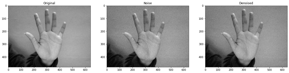
2. cv2.fastNlMeansDenoisingMulti()

# Importing OpenCV
import cv2 as cv
 
# Importing numpy
import numpy as np
 
# Importing matplotlib.pyplot
import matplotlib.pyplot as plt
 
# Capturing video using the webcam 
cap = cv.VideoCapture(0)
 
# Creating a list of the first 5 frames captured using the webcam
img = [cap.read()[1] for i in range(5)] 
 
# Converting all the images in the sequence to grayscale
gray = [cv.cvtColor(i, cv.COLOR_BGR2GRAY) for i in img]
 
# Converting the images in the sequence to float64
gray = [np.float64(i) for i in gray]
 
# Creating a noise to be added to the image for denoising
noise = np.random.randn(*gray[1].shape)*10
 
# Adding the noise to each image
noisy = [i+noise for i in gray]
 
# Converting the image back to uint8 
noisy = [np.uint8(np.clip(i,0,255)) for i in noisy]
 
# Denoising an image using the cv2.fastNlMeansDenoisingMulti function
dst = cv.fastNlMeansDenoisingMulti(noisy, 2, 5, None, 4, 7, 35)
 
# Setting the grid size
plt.figure(figsize=(20,20))
 
# Plotting the original image, the image with added noise and image after denoising operation
plt.subplot(131)
plt.title('Original')
plt.imshow(gray[2],'gray')
 
plt.subplot(132)
plt.title('Noise')
plt.imshow(noisy[2],'gray')
 
plt.subplot(133)
plt.title('Denoised')
plt.imshow(dst,'gray')

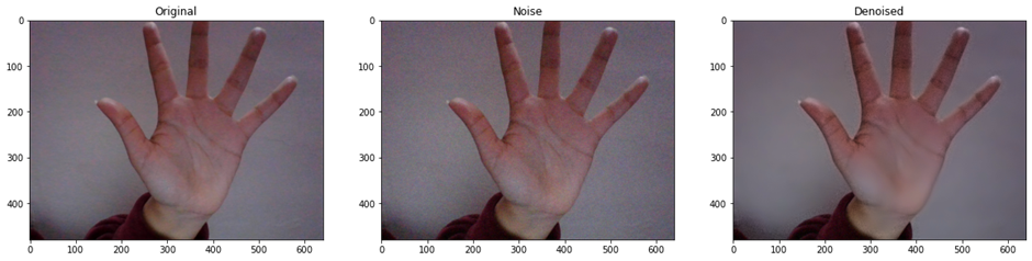
3. cv2.fastNlMeansDenoisingColoredMulti() function

# Importing OpenCV
import cv2 as cv
 
# Importing numpy
import numpy as np
 
# Importing matplotlib.pyplot
import matplotlib.pyplot as plt
 
# Capturing video using the webcam 
cap = cv.VideoCapture(0)
 
# Creating a list of the first 5 frames captured using the webcam
img = [cap.read()[1] for i in range(5)] 
 
# Converting all the images in the sequence to RGB
colored = [cv.cvtColor(i, cv.COLOR_BGR2RGB) for i in img]
 
# Converting the images in the sequence to float64
colored = [np.float64(i) for i in colored]
 
# Creating a noise to be added to the image for denoising
noise = np.random.randn(*colored[2].shape)*10
 
# Adding the noise to each image
noisy = [i+noise for i in colored]
 
# Converting the image back to uint8 
noisy = [np.uint8(np.clip(i,0,255)) for i in noisy]
 
# Denoising an image using the cv2.fastNlMeansDenoisingColoredMulti function
dst = cv.fastNlMeansDenoisingColoredMulti(noisy, 2, 5, None, 4, 7, 35)
 
# Setting the grid size
plt.figure(figsize=(20,20))
 
# Plotting the original image, the image with added noise and image after denoising operation
plt.subplot(131)
plt.title('Original')
plt.imshow(cv2.cvtColor(img[2], cv2.COLOR_BGR2RGB))
 
plt.subplot(132)
plt.title('Noise')
plt.imshow(noisy[2])
 
plt.subplot(133)
plt.title('Denoised')
plt.imshow(dst)

Conclusion

In this article, we understood what morphological operations are in OpenCV. We learned about two types of morphological operations; dilation and erosion. We understood their functioning, key differences, implementation and application. Then we understood the log transformation function in OpenCV and saw how values for pixels are computed. Furthermore, we learned about the Linear piecewise transformation function and implemented contrast stretching using it. We also explored the denoising functions in OpenCV and thoroughly understood their implementations.