Image Processing In Python

We all would have cropped our photos, rotated them, added some filters, etc. Have you ever thought of doing these by using your code? In this article, you will be able to get insights into the concept of image processing using Python. We will see different libraries Python provides for this purpose. Then we will discuss in detail the libraries numpy, scipy, OpenCV, and PIL.

Introduction to Image Processing in Python

Before discussing processing an image, let us know what does an image means?
Image is a 2D array or a matrix containing the pixel values arranged in rows and columns. Think of it as a function F(x,y) in a coordinate system holding the value of the pixel at point (x,y).

For a grayscale, the pixel values lie in the range of (0,255). And a color image has three channels representing the RGB values at each pixel (x,y), each varying from 0 to 255. It now becomes a 3-dimensional array.

Image processing, as the name suggests, is a method of doing some operation(s) on the image. You would have also heard of another term called ‘Computer Vision. The difference is that in image processing we take an input image, do required changes, and output the resulting image. Whereas, in Computer vision, we look for some features or any other information related to the input image.

Different actions are performed on the images for different applications which include cropping, flipping, rotation, segmentation, etc. Python provides functions for all these methods, using which we can set parameters that suit our needs. There are different modules in Python which contain image processing tools.

Some of these are:
1. NumPy and Scipy
2. OpenCV
3. Scikit
4. PIL/Pillow
5. SimpleCV
6. Mahotas
7. SimpleI TK
8. pgmagick
9. Pycairo

Of these, the first 5 modules are widely used by the programmers and we will be discussing numpy, scipy, OpenCV, and PIL further in the article.

Installation

As these libraries are not available directly when Python is installed, we need to install them separately before use. Since we will be using the matplotlib library to view the images, let us install it too. The following commands can help in the installation of the required libraries.

pip install numpy

pip install scipy

pip install opencv-python

pip install pillow

pip install matplotlib

NumPy and SciPy modules

NumPy and SciPy combined can be used to do image processing. Let us discuss some of the methods these modules provide for this purpose.

Reading and Saving Images

Before doing any operation on an image, we first need to load the image. So, let us see how to do that.
Example of opening an image:

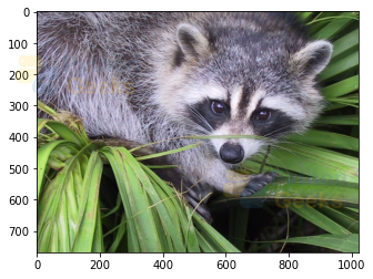
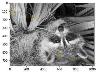
import numpy as np
from scipy import misc
import matplotlib.pyplot as plt

pic=misc.face() #reading an image from misc in scipy
plt.imshow(pic) #displaying the image using imshow() function in matplot

Output:

We can also read and save the images using misc in scipy. But these functions are depreciated in the versions of scipy above 1.2.0. The syntax of these functions are:

pic=misc.imread(location_of_image) 

misc.imsave(‘picture_name_to_be_stored’,pic) #here pic is the name of the variable holding the image

We can import more than one image from a file using the glob module. The below code shows an example of reading multiple images in the location “D:/New folder/”.

Example of reading images using glob:

import numpy as np
import cv2
import glob
from scipy import misc

path = glob.glob("D:/New folder/*.png") #storing the location of all the images in variable path
imgs = [] #creating an empty list
for img in path: #running a loop to iterate through every image in the file
    pic = plt.imread(img) #reading the image using matplotlib
    imgs.append(pic) #adding the image to the list

Cropping the image

Let us first check the type of matrix, the image gets stored in.
Example of checking the type of image matrix:

import numpy as np
from scipy import misc
import matplotlib.pyplot as plt

pic=misc.face(gray=True) # getting the image in grayscale format
type(pic)

Output:

We can see that it is a numpy array. So, we can do all the operations we do on the numpy matrices. The below code gives an example of getting a pixel value at a position.

Example of getting a pixel value:

pic[100][100]

Output:

Similarly, we can do cropping by using the concept of slicing. For example,

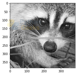
Example of cropping the image:

l=int(len(pic)/4)
crop_pic=pic[l:3*l,2*l:4*l] #taking oly some values of the matrix pic
plt.imshow(crop_pic,cmap='gray')

Output:

Getting Statistical information

As we have seen above that the image is stored in the form of a numpy array, we can apply statistical functions like max, min on the image too. Let us see the example,

Example of rotating the image:

pic=misc.face(gray=True)
print("Mean:",pic.mean())
print("Max:",pic.max())
print("Min:",pic.min())

Output:

Rotating the image

We can rotate the image using the rotate() function in the scipy module. The below example shows the way of doing it.

Example of rotating the image:

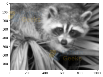
from scipy import ndimage

rot_pic=ndimage.rotate(pic,45)
plt.imshow(rot_pic,cmap='gray')

Output:

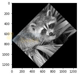
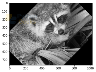
We can see in the image that its size changed to fit the rectangular block around. We can set another parameter ‘reshape’ in the rotate function to not change its size. For example,

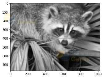
Example of rotating the image without changing the shape:

from scipy import ndimage

rot_pic=ndimage.rotate(pic,45,reshape=False)
plt.imshow(rot_pic,cmap='gray')

Output:

We can also flip the image using the flipud() function in numpy. For example,

Example of flipping the image in Python:

from scipy import ndimage

flip_pic=np.flipud(pic)
plt.imshow(flip_pic,cmap='gray')

Output:

Applying Filters on the image

The filters are mainly applied to remove the noise, blur or smoothen, or sharpen the images. Two of the most widely used filters are Gaussian and Median.

Let us see what happens when we apply a Gaussian filter to the image.

Example of applying Gaussian filter the image:

import numpy as np
from scipy import misc
import matplotlib.pyplot as plt

pic=misc.face(gray=True).astype('float') #reading the image with all the pixels considered as float values
gauss_pic=ndimage.gaussian_filter(pic,5) #specifying the sigma value of the gaussian filter as 5
plt.imshow(gauss_pic,cmap='gray')

Output:

We can see that the image got blurred. Now let us see how to sharpen the image.

Example of sharpening the image:

gauss_filter_pic=ndimage.gaussian_filter(gauss_pic,1)
sharp_pic=gauss_pic+30*(gauss_pic-gauss_filter_pic)
plt.imshow(sharp_pic,cmap='gray')

Output:

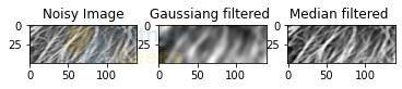
Now let us add some noise to the image and filter using both gaussian and median filters.

Example of denoising the image:

fig=plt.figure()
p=pic[100:150,10:150]
noisy_pic=p+0.7*p.std()*np.random.random(p.shape) #adding random noise to the image

ax1=fig.add_subplot(1,3,1)
ax1.imshow(noisy_pic,cmap='gray')
ax1.title.set_text("Noisy Image")

gauss_pic=ndimage.gaussian_filter(noisy_pic,3) #adding the gaussian filter
ax2=fig.add_subplot(1,3,2)
ax2.imshow(gauss_pic,cmap='gray')
ax2.title.set_text("Gaussiang filtered ")

median_pic=ndimage.median_filter(noisy_pic,3)#adding the median filter
ax3=fig.add_subplot(1,3,3)
ax3.imshow(median_pic,cmap='gray')
ax3.title.set_text("Median filtered ")

Output

Extracting Features of the image

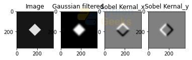
These modules also allow extracting features of the image by edge detection, segmentation, etc. Let us see some examples. For the edge detection purpose we can apply the sobel kernel.

Example of edge detection:

pic=np.zeros((256,256)) #creating a numpy array with zero values
l=int(len(pic)/3) 
pic[l:2*l,l:2*l]=1 #setting some of the pixels are 1 to form binary image
pic=ndimage.rotate(pic,45) #rotating the image

fig=plt.figure()

ax1=fig.add_subplot(1,4,1)
ax1.imshow(pic,cmap='gray')
ax1.title.set_text("Image")

pic=ndimage.gaussian_filter(pic,8) #adding gaussian filter

ax2=fig.add_subplot(1,4,2)
ax2.imshow(pic,cmap='gray')
ax2.title.set_text("Gaussian filtered ")

sobel_x=ndimage.sobel(pic,axis=0,mode='constant') #adding sobel kernel along x axis (0)

ax3=fig.add_subplot(1,4,3)
ax3.imshow(sobel_x,cmap='gray')
ax3.title.set_text("Sobel Kernal_x")

sobel_y=ndimage.sobel(pic,axis=1,mode='constant') #adding sobel kernel along y axis (1)

ax3=fig.add_subplot(1,4,4)
ax3.imshow(sobel_y,cmap='gray')
ax3.title.set_text("Sobel Kernal_y")

Output:

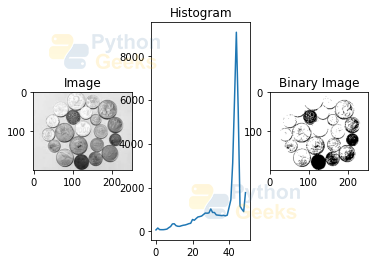
Similarly, we can do segmentation by getting the histogram and setting a threshold to form the binary image. For example,

Example of segmenting the image:

import matplotlib.image as img

pic=img.imread("D:/coins.jpg") #reading image from the desktop
pic=pic[:,:,0] #converting the image to grayscale

fig=plt.figure()

ax1=fig.add_subplot(1,3,1)
ax1.imshow(pic,cmap='gray')
ax1.title.set_text("Image")

hist,bin_edgs=np.histogram(pic,bins=50) #getting the histogram of the image

ax2=fig.add_subplot(1,3,2)
ax2.plot(hist)
ax2.title.set_text("Histogram")

bin_c=0.5*(bin_edgs[:-1]+bin_edgs[1:]) #getting all the centres of the bins of the histogram
th=sum(bin_c)/len(bin_c) #setting the threshold as average of all the bin centres

binary_img=pic>th #forming the binary image

ax2=fig.add_subplot(1,3,3)
ax2.imshow(binary_img,cmap='gray')
ax2.title.set_text("Binary Image")

Output:

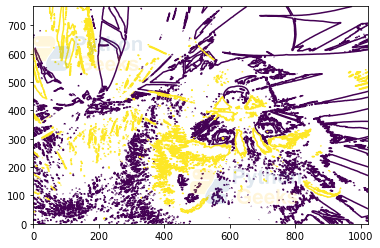
Drawing Contours on the image

We can use the counter() function to draw the counters on the image. For example,

Example of segmenting the image:

pic=misc.face(gray=True).astype('float')
plt.contour(pic,[60,200])

Output:

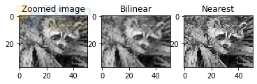
Interpolation in Python

Interpolation is the process of finding the unknown value that occurs between the known values. In the case of an image, we apply interpolation when we zoom the image. As we need to give more pixel values than the original image and for this purpose, we need to find the intermediate pixel values. The interpolation provides many options like bilinear, nearest, etc. Let us see what happens when we use these options.

Example of interpolating the image:

pic=misc.face(gray=True)
zoom_pic=ndimage.zoom(pic,0.05)

fig=plt.figure()

ax1=fig.add_subplot(1,3,1)
ax1.imshow(zoom_pic,cmap='gray')
ax1.title.set_text("Zoomed image")

ax2=fig.add_subplot(1,3,2)
ax2.imshow(zoom_pic,cmap=plt.cm.gray,interpolation='bilinear')
ax2.title.set_text("Bilinear")

ax2=fig.add_subplot(1,3,3)
ax2.imshow(zoom_pic,cmap=plt.cm.gray,interpolation='nearest')
ax2.title.set_text("Nearest")

Output:

OpenCV

OpenCV is also another image processing library. It contains various functions to do processing of the images and extract required features. Let us discuss some of them.

Reading and Saving the image

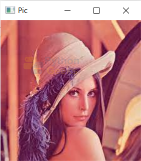
We can read the image using the imread() method. The below code gives an example.

Example of reading an image:

import cv2

pic = cv2.imread("D:/lena.png")
cv2.imshow("Pic",pic)
cv2.waitKey(0) #waits till close option is clicked
cv2.destroyAllWindows()  #closing all the windows on closing the picture

Output:

And to save the image we use the imwrite() function using the below syntax.

cv2.imwrite(filename, image)

We can also find information about the image like size, dimensions, etc. For example,

Example of getting information about the image:

print("No. of Pixels: ",pic.size)

print("Dimension: ",pic.shape)

Output:

We got three values in the dimension as there are three channels in the color image.

Splitting the Channels

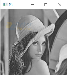
We can get the grayscale image using the ‘cv2.IMREAD_GRAYSCALE’ parameter while reading the image as shown below.

Example of reading the image as grayscale:

import cv2

pic = cv2.imread("D:/lena.png",cv2.IMREAD_GRAYSCALE)
cv2.imshow("Pic",pic)
cv2.waitKey(0) 
cv2.destroyAllWindows()  

Output:

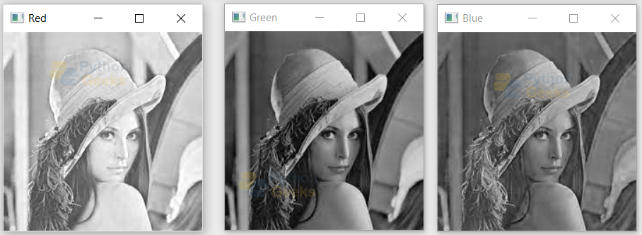
And we can get the blue, green, red channels using the split() function. Let us split them and see the results.

Example of splitting the image:

import cv2

pic = cv2.imread("D:/lena.png")
(B, G, R) = cv2.split(pic)

cv2.imshow("Red", R)
cv2.imshow("Green", G)
cv2.imshow("Blue", B)
cv2.waitKey(0)
cv2.waitKey(0) 
cv2.destroyAllWindows()  

Output:

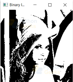
Binarization

We can convert the image into a binary image using the threshold() function. For example,

Example of binarizing the image:

gray_pic = cv2.cvtColor(pic, cv2.COLOR_BGR2GRAY) #converting the image into grayscale
r, threshold = cv2.threshold(gray_pic, 125, 255, cv2.THRESH_OTSU) #converting the image into grayscale using the histogram method
cv2.imshow('Binary Image',threshold)
cv2.waitKey(0) 
cv2.destroyAllWindows()  

Output:

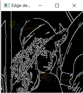
Edge Detection

Edges are the borders of different parts of the image that lets us differentiate these parts. When we talk in terms of a digital image, edges are the pixels where there is a sudden change in the pixel values. OpenCV contains a function called canny() to detect the edges. The below codes give an example.

Example of edge detection :

import cv2

pic = cv2.imread("D:/lena.png")
gray_pic = cv2.cvtColor(pic, cv2.COLOR_BGR2GRAY)

edges_pic = cv2.Canny(pic, 100,200) #getting the image with edges detected

cv2.imshow("Edge detection",edges_pic)
cv2.waitKey(0) 
cv2.destroyAllWindows() 

Output:

PIL

Opening and Saving the Image

We can read the image using the open() function. For example,
Example of reading an image:

from PIL import Image

pic = Image.open("D:/pic.png")
pic.show()

Output:

We can save the image save method as shown below.
Example of saving the image:

pic.save("newImage.png")

We can also get information about the image like size, format, etc.
Example of getting information about the image:

print(pic)
print("size:",pic.size)
print("format:",pic.format)

Output:

Convert to grayscale

We can use the convert() method to convert it to a grayscale image. For example,
Example of converting the image into grayscale:

gray_pic=pic.convert('L')
gray_pic

Output:

Rotating

We can use the rotate() function to rotate the image by a specified angle in an anticlockwise direction. For example,
Example of rotating the image:

pic.rotate(45)

Output:

Resize

Unlike the above operation, we do not use any resize() function here! Instead, we use the function named thumbnail() and give the input of the required size.
Example of resizing the image:

pic.thumbnail((200,300))
pic

Output:

Quiz on Image Processing in Python

Conclusion

In this article, we discussed image processing, different modules in Python that help in applying different methods to the images. We covered NumPY, SciPy, OpenCV, and PIL modules.

Hope you enjoyed reading this article. Happy learning!